





ML Models Built on Google Cloud Solutions Help You Virtually Participate in National Muffin Day!

2949
Of your peers have already read this article.
2:00 Minutes
The most insightful time you'll spend today!
If you’re here you’re probably wondering: what on Earth is the connection between muffins and machine learning, and what is National Muffin Day? To understand this, let’s start with National Muffin Day: an annual holiday co-founded by Jacob and his friend Julia Levy in 2015 to bake muffins and raise money for homelessness. National Muffin Day will occur on Sunday, February 20 this year. For more information on how to participate in National Muffin Day (which involves delicious baked goods and donations to people in need), please see the information at the bottom of this post. Last year, a colleague connected Jacob with Sara, who had done several baking projects that used machine learning to generate new recipes. They decided to collaborate for this year’s National Muffin Day, adding a new muffin recipe created with the help of machine learning.
In this post, we’ll explain how Sara used Google Cloud to develop a new muffin recipe, show you how you can participate virtually in National Muffin Day, and of course—share the recipe.
Machine learning for muffins
At its core, machine learning is the process of finding patterns in data and using those patterns to make predictions on new data. After a lot of baking over the past few years, Sara learned that baking is also based on patterns. For example, the ratio of flour, fat, liquid, and sugar that make up a cookie is very different from the ratio of those ingredients for a bread, a pie crust, or a muffin. She used that discovery to create a recipe for a hybrid cake + cookie, and a cake filled with Maltesers. Next up: muffins!
The first step was figuring out how to translate the task of generating a new muffin recipe into a machine learning task. To solve this, she planned to use numerical data on the amounts of different ingredients in a muffin recipe to train the model. Sara considered two types of models for this task: classification and regression. A classification model would categorize muffin recipes into different muffin types based on their ingredient amounts, and a regression model would do the reverse: take a type of muffin and return the amount of each ingredient needed to make it. She decided to build a regression model, since it would be more fun for the model to return ingredient amounts, rather than tell you which type of muffin recipe you’re already making.
Implementing this first required identifying a few muffin categories and collecting recipe data. This presented a new challenge, since her previous baking models used categories for distinct baked goods (i.e. cakes, cookies, breads). After scouring through quite a few recipes, Sara discovered that many muffins fall into two types: those that use only traditional ingredients as their base (flour, sugar, butter, milk, etc.), and those that include an alternative ingredient, most commonly a pureed fruit, to make the base (like bananas, applesauce, or pumpkin). Using those two categories, the model would take the type of muffin as input and return the amounts of base ingredients required to make that recipe. Here, the inputs can be any values adding up to 100%:
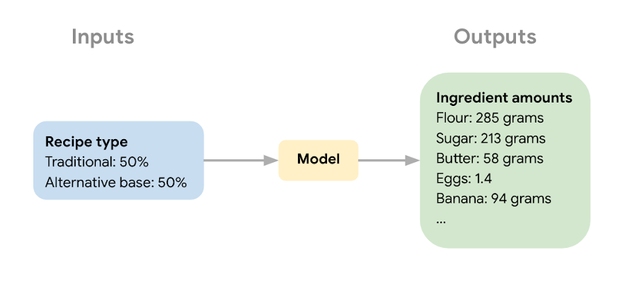
The next step in the ML process was collecting recipe data to use for model training and narrowing down the ingredients used to train the model. Sara wanted the model to learn the combination of core ingredients that make up a muffin batter, rather than flavorings and additions like blueberries, vanilla extract, or chocolate chips. These tasty additions could be added after the model helped create the muffin batter. Once she gathered enough recipes, she removed extra ingredients for training purposes and converted ingredients from different recipes into the same unit (grams, milliliters, and teaspoons).
Building a muffin model with Vertex AI
Sara uploaded the muffin ingredient data into BigQuery, and then created a notebook instance in Vertex AI Workbench to analyze the data. With the new Workbench managed instances, you can interactively query BigQuery tables directly from your instance and copy the code to download your data to a notebook as a Pandas DataFrame:
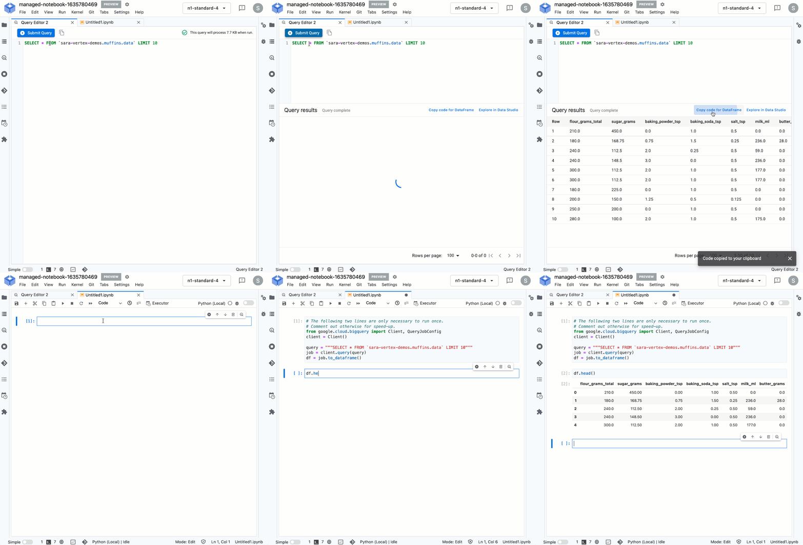
From her notebook instance, Sara experimented with different ML frameworks and model types. She landed on a Scikit-learn regression model to solve this task, and to mimic a real-world production environment, decided to convert this workflow into a ML pipeline. Using the Kubeflow Pipelines SDK, she ran the following on Vertex Pipelines:
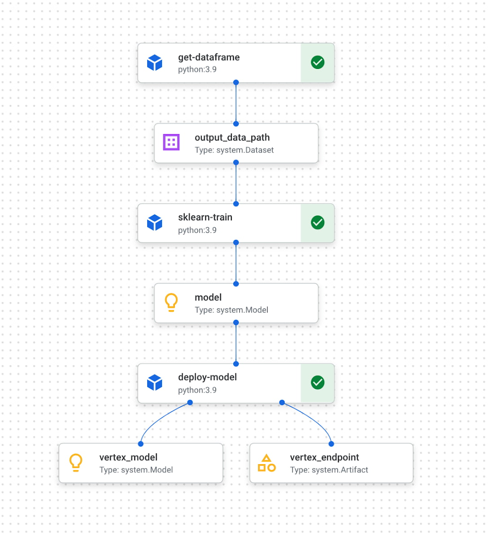
The first component reads the ingredient data from BigQuery and converts it into a Pandas DataFrame which is passed to the next pipeline step. In this step, we train a custom Scikit-learn model on the recipe data. Finally, this model is deployed to an endpoint in Vertex AI. To put it all together, Sara built a web app that allowed her to easily generate ingredient amounts for different muffin types. The web app uses the Vertex AI SDK to call the deployed model endpoint and return ingredient amounts.
The recipe
With a deployed recipe generation model, the only thing left to do was test recipes in the kitchen! Because the model only returns ingredient amounts, there were still many key human elements to complete the baking process: adding yummy additions to the core muffin batter, making adjustments to optimize taste, determining the method for adding ingredients, baking time, and more. After testing a few recipes generated by the model, we landed on a favorite which we’re very excited to share with you here.
Berry ML Muffins

Makes 12 muffins
Flour 285 grams (2 cups)
Granulated sugar 250 grams (1 cup)
Baking powder 2 teaspoons
Baking soda ¼ teaspoon
Salt ½ teaspoon
Cinnamon ½ teaspoon
Milk 170 ml (⅔ cup), room temperature
Butter 55 grams (¼ cup), melted and slightly cooled
Eggs 1 egg plus 1 egg white, room temperature
Canola or vegetable oil 50 grams (¼ cup)
Sour cream 50 grams (3 tablespoons + ¾ teaspoon), room temperature
Vanilla extract 1 ½ teaspoons
Blueberries or raspberries 240 grams (1 ½ cups)
Coarse sugar, like demerara or turbinado (optional for topping) 1 tablespoon
- Measure your three cold ingredients and allow them to come to room temperature: 1 egg + 1 egg white, sour cream, and milk.
- Preheat the oven to 375 F / 190 C. Line a 12-muffin tin with cupcake liners or lightly grease with baking spray.
- In a large bowl, whisk together flour, baking powder, baking soda, salt, and cinnamon. Set aside.
- Melt your butter in a medium heat proof bowl, and allow it to cool slightly for a few minutes. Whisk in sugar until combined. Then add egg, oil, and vanilla, milk, and sour cream and whisk until fully incorporated.
- Pour the wet ingredients into the dry ingredients, mixing with a spatula until just combined. Be careful not to overmix, it’s ok if there are a few lumps in your batter.
- Prepare your fruit. If you can’t decide whether to use blueberries or raspberries, divide your batter into two bowls and do both! Crush half of your fruit and fold it into the batter. Then mix in the remaining whole berries.
- Divide the mixture evenly into the muffin tin. Optionally (but extra tasty), sprinkle the tops of each muffin with about ⅛ teaspoon of coarse sugar. Turbinado or demerara sugar work well for this. This will caramelize and add a nice texture to the tops of your muffins.
- Bake at 375 for 22 – 24 minutes, or until a toothpick inserted in the center comes out clean. For best results, do a toothpick test in a few muffins since not all ovens have an even temperature throughout. Let the muffins cool in the muffin tin for a few minutes, then transfer to a wire rack to cool completely.
- Enjoy!
How can you participate in National Muffin Day?
Participation in National Muffin Day is as easy as 1-2-3!
- On February 20, Bake Muffins. It’s time to dust those muffin tins, grab your blueberries, chocolate chips, rhubarb, and favorite ingredients, and create some magical scrumdiddlyumptiousness! If you want to join Jacob in a virtual baking party, you can register here.
- Then, Give. In non-pandemic years, we asked our bakers to personally hand muffins to hungry folks in their cities. While this is a valuable and rewarding experience, the current state of Covid means this practice is still unsafe, so we request that you refrain from doing this. Instead, if it feels safe, we encourage you to take your delicious baked goods and donate them to local homeless shelters, which can distribute them to those in need. Alternatively, you can share your muffins with friends and families and then make a donation to an organization that benefits people experiencing homelessness, like the ones listed below in step 3.
- Share Your Muffin Pics on Social Media. We’d love to see your muffins! Share your pictures on Twitter or Instagram with the hashtags #givemuffins, or share them to our official Facebook Event page. For each individual baker who participates, we will make donations to Project Homeless Connect, which provides much needed resources to people experiencing homelessness in San Francisco, Family promise, which supports unhoused families nationwide, and Pine Street Inn which provides resources for people experiencing homelessness in Boston. Donations will be on a per-baker basis (with up to $80 donated per baker!), so please feel free to loop in your significant others, kids, nieces and nephews, roommates, friends, and anybody else with a giving spirit who loves deliciousness!
BigQuery Explainable AI for Demystifying the Inner Workings of ML Models. Now GA!

6551
Of your peers have already read this article.
2:00 Minutes
The most insightful time you'll spend today!
Explainable AI (XAI) helps you understand and interpret how your machine learning models make decisions. We’re excited to announce that BigQuery Explainable AI is now generally available (GA). BigQuery is the data warehouse that supports explainable AI in a most comprehensive way w.r.t both XAI methodology and model types. It does this at BigQuery scale, enabling millions of explanations within seconds with a single SQL query.
Why is Explainable AI so important? To demystify the inner workings of machine learning models, Explainable AI is quickly becoming an essential and growing need for businesses as they continue to invest in AI and ML. With 76% of enterprises now prioritizing artificial intelligence (AI) and machine learning (ML) over other initiatives in 2021 IT budgets, the majority of CEOs (82%) believe that AI-based decisions must be explainable to be trusted according to a PwC survey.
While the focus of this blogpost is on BigQuery Explainable AI, Google Cloud provides a variety of tools and frameworks to help you interpret models outside of BigQuery, such as with Vertex Explainable AI, which includes AutoML Tables, AutoML Vision, and custom-trained models.
So how does Explainable AI in BigQuery work exactly? And how might you use it in practice?
Two types of Explainable AI: global and local explainability
When it comes to Explainable AI, the first thing to note is that there are two main types of explainability as they relate to the features used to train the ML model: global explainability and local explainability.
Imagine that you have a ML model that predicts housing price (as a dollar amount), based on three features: (1) number of bedrooms, (2) distance to the nearest city center, and (3) construction date.
Global explainability (a.k.a. global feature importance) describes the features’ overall influence on the model and helps you understand if a feature had a greater influence than other features over the model’s predictions. For example, global explainability can reveal that the number of bedrooms and distance to city center typically has a much stronger influence than the construction date on predicting housing prices. Global explainability is especially useful if you have hundreds or thousands of features and you want to determine which features are the most important contributors to your model. You may also consider using global explainability as a way to identify and prune less important features to improve the generalizability of their models.
Local explainability (a.k.a. feature attributions) describes the breakdown of how each feature contributes towards a specific prediction. For example, if the model predicts that house ID#1001 has a predicted price of $230,000, local explainability would describe a baseline amount (e.g. $50,000) and how each of the features contributes on top of the baseline towards the predicted price. For example, the model may say that on top of the baseline of $50,000, having 3 bedrooms contributed an additional $50,000, close proximity to the city center added $100,000, and construction date of 2010 added $30,000, for a total predicted price of $230,000. In essence, understanding the exact contribution of each feature used by the model to make each prediction is the main purpose of local explainability.
What ML models does BigQuery Explainable AI apply to?
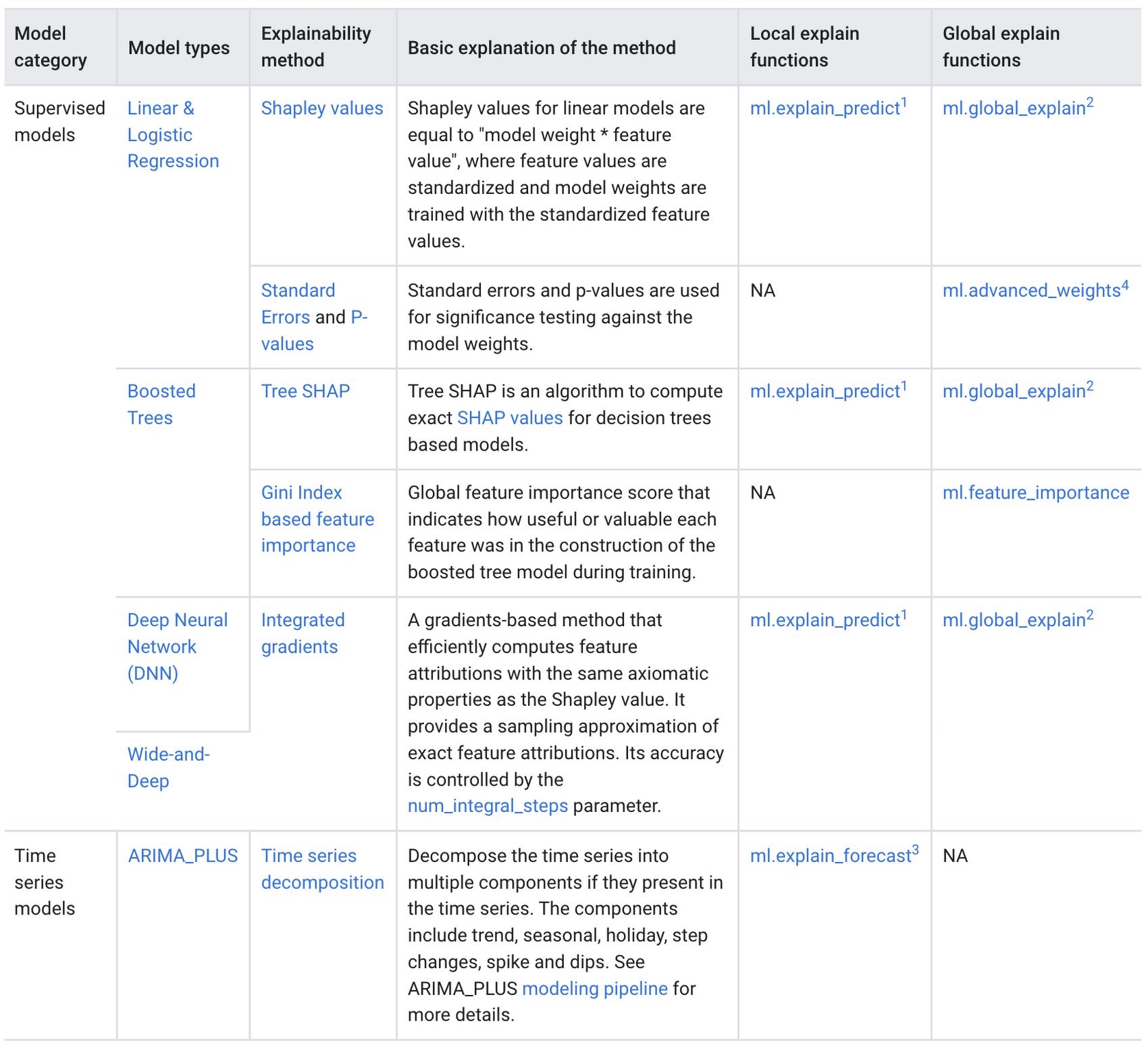
BigQuery Explainable AI applies to a variety of models, including supervised learning models for IID data and time series models. The documentation for BigQuery Explainable AI provides an overview of the different ways of applying explainability per model. Note that each explainability method has its own way of calculation (e.g. Shapley values), which are covered more in-depth in the documentation.
Examples with BigQuery Explainable AI
In this next section, we will show three examples of how to use BigQuery Explainable AI in different ML applications:
Regression models with BigQuery Explainable AI
Let’s use a boosted tree regression model to predict how much a taxi cab driver will receive in tips for a taxi ride, based on features such as number of passengers, payment type, total payment and trip distance. Then let’s use BigQuery Explainable AI to help us understand how the model made the predictions in terms of global explainability (which features were most important?) and local explainability (how did the model arrive at each prediction?).
The taxi trips dataset comes from the BigQuery public datasets and is publicly available in the table: bigquery-public-data.new_york_taxi_trips.tlc_yellow_trips_2018.
First, you can train a boosted tree regression model.
CREATE OR REPLACE MODEL bqml_tutorial.taxi_tip_regression_modelOPTIONS (model_type='boosted_tree_regressor',input_label_cols=['tip_amount'],max_iterations = 50,tree_method = 'HIST',subsample = 0.85,enable_global_explain = TRUE) ASSELECTvendor_id,passenger_count,trip_distance,rate_code,payment_type,total_amount,tip_amountFROM`bigquery-public-data.new_york_taxi_trips.tlc_yellow_trips_2018`WHERE tip_amount >= 0LIMIT 1000000
Now let’s do a prediction using ML.PREDICT, which is the standard way in BigQuery ML to make predictions without explainability.
SELECT *FROMML.PREDICT(MODEL bqml_tutorial.taxi_tip_regression_model,(SELECT"0" AS vendor_id,1 AS passenger_count,CAST(5.85 AS NUMERIC) AS trip_distance,"0" AS rate_code,"0" AS payment_type,CAST(55.56 AS NUMERIC) AS total_amount))

But you might wonder—how did the model generate this prediction of ~11.077?
BigQuery Explainable AI can help us answer this question. Instead of using ML.PREDICT, you use ML.EXPLAIN_PREDICT with an additional optional parameter top_k_features. ML.EXPLAIN_PREDICT extends the capabilities of ML.PREDICT by outputting several additional columns that explain how each feature contributes to the predicted value. In fact, since ML.EXPLAIN_PREDICT includes all the output from ML.PREDICT anyway, you may want to consider using ML.EXPLAIN_PREDICT every time instead.
SELECT *FROMML.EXPLAIN_PREDICT(MODEL bqml_tutorial.taxi_tip_regression_model,(SELECT"0" AS vendor_id,1 AS passenger_count,CAST(5.85 AS NUMERIC) AS trip_distance,"0" AS rate_code,"0" AS payment_type,CAST(55.56 AS NUMERIC) AS total_amount),STRUCT(6 AS top_k_features))
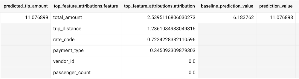
The way to interpret these columns is:
Σfeature_attributions + baseline_prediction_value = prediction_value
Let’s break this down. The prediction_value is ~11.077, which is simply the predicted_tip_amount. The baseline_prediction_value is ~6.184, which is the tip amount for an average instance. top_feature_attributions indicates how much each of the features contributes towards the prediction value. For example, total_amount contributes ~2.540 to the predicted_tip_amount.
ML.EXPLAIN_PREDICT provides local feature explainability for regression models. For global feature importance, see the documentation for ML.GLOBAL_EXPLAIN.
Classification models with BigQuery Explainable AI
Let’s use a logistic regression model to show you an example of BigQuery Explainable AI with classification models. We can use the same public dataset as before: bigquery-public-data.new_york_taxi_trips.tlc_yellow_trips_2018.
Train a logistic regression model to predict the bracket of the percentage of the tip amount out of the taxi bill.
CREATE OR REPLACE MODEL bqml_tutorial.taxi_tip_classification_modelOPTIONS(model_type='logistic_reg',input_label_cols=['tip_bucket'],enable_global_explain=true) ASSELECTvendor_id,passenger_count,trip_distance,rate_code,payment_type,total_amount,CASEWHEN tip_amount > total_amount*0.20 THEN '20% or more'WHEN tip_amount > total_amount*0.15 THEN '15% to 20%'WHEN tip_amount > total_amount*0.10 THEN '10% to 15%'ELSE '10% or less'END AS tip_bucketFROM`bigquery-public-data.new_york_taxi_trips.tlc_yellow_trips_2018`WHERE tip_amount >= 0LIMIT 1000000
Next, you can run ML.EXPLAIN_PREDICT to get both the classification results and the additional information for local feature explainability. For global explainability, you can use ML.GLOBAL_EXPLAIN. Again, since ML.EXPLAIN_PREDICT includes all the output from ML.PREDICT anyway, you may want to consider using ML.EXPLAIN_PREDICT every time instead.
SELECT *FROMML.EXPLAIN_PREDICT(MODEL bqml_tutorial.taxi_tip_classification_model,(SELECT"0" AS vendor_id,1 AS passenger_count,CAST(5.85 AS NUMERIC) AS trip_distance,"0" AS rate_code,"0" AS payment_type,CAST(55.56 AS NUMERIC) AS total_amount),STRUCT(6 AS top_k_features))
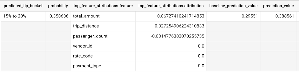
Similar to the regression example earlier, the formula is used to derive the prediction_value:
Σfeature_attributions + baseline_prediction_value = prediction_value
As you can see in the screenshot above, the baseline_prediction_value is ~0.296. total_amount is the most important feature in making this specific prediction, contributing ~0.067 to the prediction_value, though followed by trip_distance. The feature passenger_count contributes negatively to prediction_value by -0.0015. The features vendor_id, rate_code, and payment_type did not seem to contribute much to the prediction_value.
You may wonder why the prediction_value of ~0.389 doesn’t equal the probability value of ~0.359. The reason is that unlike for regression models, for classification models, prediction_value is not a probability score. Instead, prediction_value is the logit value (i.e., log-odds) for the predicted class, which you could separately convert to probabilities by applying the softmax transformation to the logit values. For example, a three-class classification has a log-odds output of [2.446, -2.021, -2.190]. After applying the softmax transformation, the probability of these class predictions is [0.9905, 0.0056, 0.0038].
Time-series forecasting models with BigQuery Explainable AI
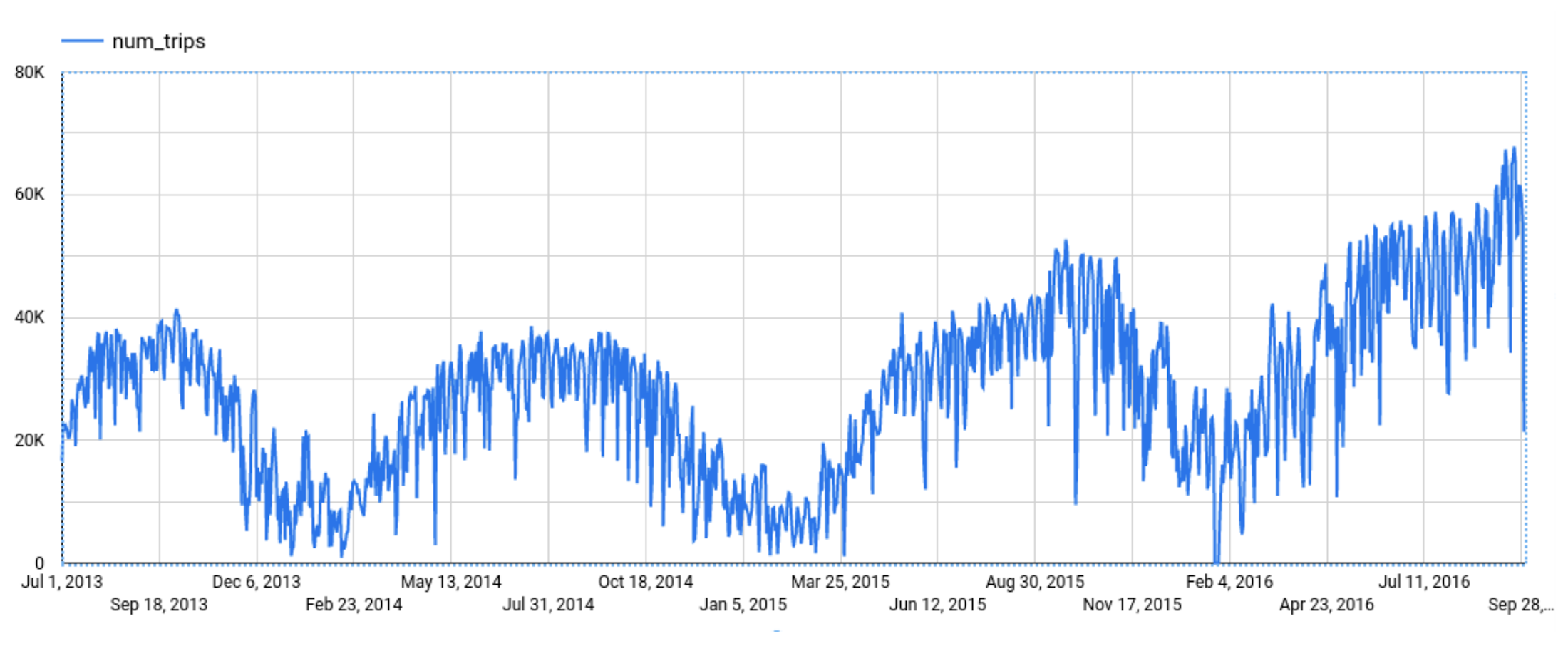
Explainable AI for forecasting provides more interpretability into how the forecasting model came to its predictions. Let’s go through an example of forecasting the number of bike trips in NYC using the new_york.citibike_trips public data in BigQuery.
You can train a time-series model ARIMA_PLUS:
CREATE OR REPLACE MODEL bqml_tutorial.nyc_citibike_arima_modelOPTIONS(model_type = 'ARIMA_PLUS',time_series_timestamp_col = 'date',time_series_data_col = 'num_trips',holiday_region = 'US') ASSELECTEXTRACT(DATE from starttime) AS date,COUNT(*) AS num_tripsFROM`bigquery-public-data.new_york.citibike_trips`GROUP BY dateNext, you can first try forecasting without explainability using ML.FORECAST:SELECT*FROMML.FORECAST(MODEL bqml_tutorial.nyc_citibike_arima_model,STRUCT(365 AS horizon, 0.9 AS confidence_level))
This function outputs the forecasted values and the prediction interval. Plotting it in addition to the input time series gives the following figure.
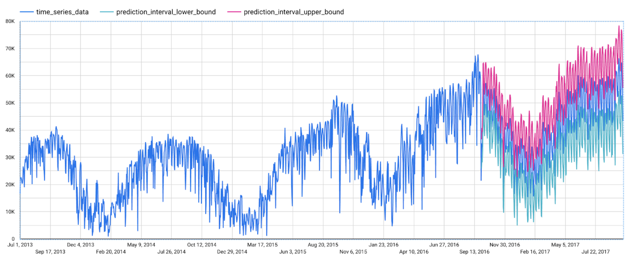
But how does the forecasting model arrive at its predictions? Explainability is especially important if the model ever generates unexpected results.
With ML.EXPLAIN_FORECAST, BigQuery Explainable AI provides extra transparency into the seasonality, trend, holiday effects, level (step) changes, and spikes and dips outlier removal. In fact, since ML.EXPLAIN_FORECAST includes all the output from ML.FORECAST anyway, you may want to consider using ML.EXPLAIN_FORECAST every time instead.
SELECT*FROMML.EXPLAIN_FORECAST(MODEL bqml_tutorial.nyc_citibike_arima_model,STRUCT(365 AS horizon, 0.9 AS confidence_level))
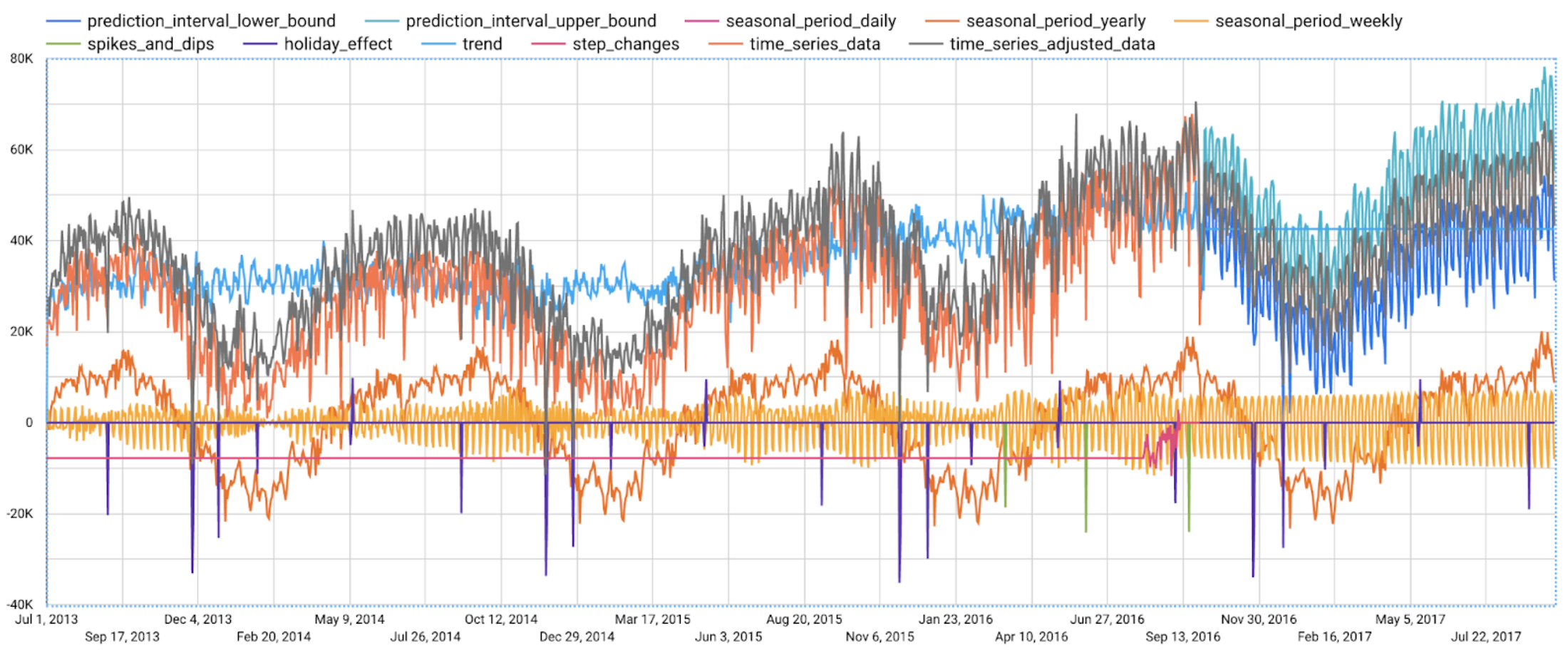
Compared to the previous figure which only shows the forecasting results, this figure shows much richer information to explain how the forecast is made.
First, it shows how the input time series is adjusted by removing the spikes and dips anomalies, and by compensating the level changes. That is:
time_series_adjusted_data = time_series_data - spikes_and_dips - step_changes
Second, it shows how the adjusted input time series is decomposed into different components such as both weekly and yearly seasonal components, holiday effect component and trend component. That is
time_series_adjusted_data = trend + seasonal_period_yearly + seasonal_period_weekly + holiday_effect + residual
Finally, it shows how these components are forecasted separately to compose the final forecasting results. That is:
time_series_data = trend + seasonal_period_yearly + seasonal_period_weekly + holiday_effect
For more information on these time series components, please see the documentation here.
Conclusion
With the GA of BigQuery Explainable AI, we hope you will now be able to interpret your machine learning models with ease.
Thanks to the BigQuery ML team, especially Lisa Yin, Jiashang Liu, Amir Hormati, Mingge Deng, Jerry Ye and Abhinav Khushraj. Also thanks to the Vertex Explainable AI team, especially David Pitman and Besim Avci.
5117
Of your peers have already watched this video.
1:47 Minutes
The most insightful time you'll spend today!
How adidas’s Marketing Team Benefits from Google Cloud Marketing Platform
We live in a world where the consumer journey is no longer linear, making it difficult to know when to deliver a brand message or a product message.
“We talk a lot about the consumer journey no longer being linear. It’s very difficult to know when the consumer is going to come in contact with your message. And because of that it makes it much harder to deliver the right message at the right time,” says Chris Murphy, Head of Digital Experience, adidas.
To solve the problem, adidas turned to the Google Cloud Marketing Platform to use audience insights to inform the art of storytelling and help teams, from brand marketing to retail to e-commerce, deliver relevant messages across channels.
“In a singular environment like Google Cloud Marketing Platform, when you’re able to see audience insights and information…we know when someone should be receiving a brand message versus a product message — when they’re thinking about buying or when they’re actually ready to purchase,” says Murphy.
It wasn’t easy at the start. “Being in brand marketing for so long, there was this initial pushback on data and the science behind it, because it was an art. But what we’re seeing now is the ability for data and insights to really inform the art of storytelling. It allows us to understand the impact that we’re having in real time,” says Kelly Olmstead, VP, Brand Activation for North America, adidas.
Today adidas’ marketing team depends more heavily on data and analysis to guide its strategy. “Starting every meeting with data and insights, that’s something that we want to take outside of just the marketing organization, and really infuse it across our culture here at adidas,” says Olmstead.
Watch how adidas benefits from using the Google Cloud Marketing Platform.
3016
Of your peers have already watched this video.
16:30 Minutes
The most insightful time you'll spend today!
Predicting Treasury Settlement Failures with ML
BNY Mellon’s Government Securities Services (GSS) business is the sole provider of treasury settlement services in the United States of America. Given its unique market position, GSS is exploring how to help clients improve their forecasting of $70+ billion in daily settlement fails leveraging Google Cloud.
Sarthak Pattanaik, Chief Information Officer, Clearance and Collateral Technology, The Bank of New York Mellon and Victor O’Laughlen, Digital Business Leader, Clearance and Collateral, The Bank of New York Mellon, share how they utilized Google Cloud AI solutions to predict treasury settlement failures.
They take us through the business process, the steps they took to set up their AI solution, and what they have learnt on their journey—not just from a technical standpoint but from a cultural one as well.
Build A Movie Recommender System based on Reinforcement Learning (RL) with Vertex AI

3330
Of your peers have already read this article.
3:00 Minutes
The most insightful time you'll spend today!
Reinforcement learning (RL) is a form of machine learning whereby an agent takes actions in an environment to maximize a given objective (a reward) over this sequence of steps. Applications of RL include learning-based robotics, autonomous vehicles and content serving. The fundamental RL system includes many states, corresponding actions, and rewards to those actions. Translate that into a movie recommender system: The ‘state’ is the user, the ‘action’ is the movie to recommend to the user, and the ‘reward’ is the user rating of the movie. RL is a great framework for optimizing ML models, as mentioned by Spotify in the keynote in the Applied ML Summit 2021.
In this article, we’ll demonstrate an RL-based movie recommender system executed in Vertex AI and built with TF-Agents, a library for RL in TensorFlow. This demo has two parts: (1) a step-by-step guide leveraging Vertex Training, Hyperparameter Tuning, and Prediction services; (2) a MLOps guide to build end-to-end pipelines using Vertex Pipelines and other Vertex services.
TF-Agents meets Vertex AI
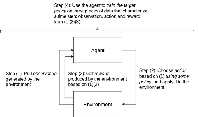
In reinforcement learning (RL), an agent takes a sequence of actions in a given environment according to some policy, with the goal of maximizing a given reward over this sequence of actions. TF-Agents is a powerful and flexible library enabling you to easily design, implement and test RL applications. It provides you with a comprehensive set of logical modules that support easy customization:
- Policy: A mapping from an environment observation to an action or a distribution over actions. It is the artifact produced from training, and the equivalent of a “Model” in a supervised learning setup.
- Action: A move or behavior that is outputted by some policy, and chosen and taken by an agent.
- Agent: An entity that encapsulates an algorithm to use one or more policies to choose and take actions, and trains the policy.
- Observations: A characterization of the environment state.
- Environment: Definition of the RL problem to solve. At each time step, the environment generates an observation, bears the effect of the agent action, and then given the action taken and the observation, the environment responds with a reward as feedback.
A typical RL training loop looks like the following:
A typical process to build, evaluate, and deploy RL applications would be:
- Frame the problem: While this blog post introduces a movie recommendation system, you can use RL to solve a wide range of problems. For instance, you can easily solve a typical classification problem with RL, where you can frame predicted classes as actions. One example would be digit classification: observations are digit images, actions are 0-9 predictions and rewards indicate whether the predictions match the ground truth digits.
- Design and implement RL simulated experiments: We will go into detail on simulated training data and prediction requests in the end-to-end pipeline demo.
- Evaluate performance of the offline experiments.
- Launch end-to-end production pipeline by replacing the simulation constituents with real-world interactions.
Now that you know how we’ll build a movie recommendation system with RL, let’s look at how we can use Vertex AI to run our RL application in the cloud. We’ll use the following Vertex AI products:
- Vertex AI training to train a RL policy (the counterpart of a model in supervised learning) at scale
- Vertex AI hyperparameter tuning to find the best hyperparameters
- Vertex AI prediction to serve trained policies at endpoints
- Vertex Pipelines to automate, monitor, and govern your RL systems by orchestrating your workflow in a serverless manner, and storing your workflow’s artifacts using Vertex ML Metadata.
Step-by-step RL demo
This step-by-step demo showcases how to build the MovieLens recommendation system using TF-Agents and Vertex AI services, primarily custom training and hyperparameter tuning, custom prediction and endpoint deployment. This demo is available on Github, including a step-by-step notebook and Python modules.
The demo first walks through the TF-Agents on-policy (which is covered in detail in the demo) training code of the RL system locally in the notebook environment. It then shows how to integrate the TF-Agents implementation with Vertex AI services: It packages the training (and hyperparameter tuning) logic in a custom training/hyperparameter tuning container and builds the container with Cloud Build. With this container, it executes remote training and hyperparameter tuning jobs using Vertex AI. It also illustrates how to utilize the best hyperparameters learned from the hyperparameter tuning job during training, as an optimization.
The demo also defines the prediction logic, which takes in observations (user vectors) from prediction requests and outputs predicted actions (movie items to recommend), in a custom prediction container and builds the container with Cloud Build. It deploys the trained policy to a Vertex AI endpoint, and uses the prediction container as the serving container for the policy at the Vertex AI endpoint.
End-to-end workflow with a closed feedback loop: Pipeline demo
Pipeline architecture
Building upon our RL demo, we’ll now show you how to scale this workflow using Vertex Pipelines. This pipeline demo showcases how to build an end-to-end MLOps pipeline for the MovieLens recommendation system, using Kubeflow Pipelines (KFP) for authoring and Vertex Pipelines for orchestration.
Highlights of this end-to-end demo include:
- RL-specific implementation that handles RL modules, training logic and trained policies as opposed to models
- Simulated training data, simulated environment for predictions and re-training
- Closing of the feedback loop from prediction results back to training
- Customizable and reproducible KFP components
An illustration of the pipeline structure is shown in the figure below.
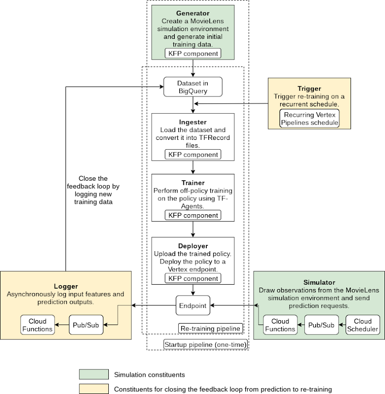
The pipeline consists of the following components:
- Generator: to generate MovieLens simulation data as the initial training dataset using a random data-collecting policy, and store in BigQuery [executed only once]
- Ingester: to ingest training data in BigQuery and output TFRecord files
- Trainer: to perform off-policy (which is covered in detail in the demo) training using the training dataset and output a trained RL policy
- Deployer: to upload the trained policy, create a Vertex AI endpoint and deploy the trained policy to the endpoint
In addition to the above pipeline, there are three components which utilize other GCP services (Cloud Functions, Cloud Scheduler, Pub/Sub):
- Simulator: to send recurring simulated MovieLens prediction requests to the endpoint
- Logger: to asynchronously log prediction inputs and results as new training data back to BigQuery, per prediction requests
- Trigger: to recurrently execute re-training on new training data
Pipeline construction with Kubeflow Pipelines (KFP)
You can author the pipeline using the individual components mentioned above:
@dsl.pipeline(pipeline_root=PIPELINE_ROOT,name=f"{PIPELINE_NAME}-startup")def pipeline(# Pipeline configsproject_id: str,raw_data_path: str,training_artifacts_dir: str,# BigQuery configsbigquery_dataset_id: str,bigquery_location: str,bigquery_table_id: str,bigquery_max_rows: int = 10000,# TF-Agents RL configsbatch_size: int = 8,rank_k: int = 20,num_actions: int = 20,driver_steps: int = 3,num_epochs: int = 5,tikhonov_weight: float = 0.01,agent_alpha: float = 10) -> None:"""Authors a RL pipeline for MovieLens movie recommendation system.Integrates the Generator, Ingester, Trainer and Deployer components. Thispipeline generates initial training data with a random policy and runs onceas the initiation of the system.Args:project_id: GCP project ID. This is required because otherwise the BigQueryclient will use the ID of the tenant GCP project created as a result ofKFP, which doesn't have proper access to BigQuery.raw_data_path: Path to MovieLens 100K's "u.data" file.training_artifacts_dir: Path to store the Trainer artifacts (trained policy).bigquery_dataset: A string of the BigQuery dataset ID in the format of"project.dataset".bigquery_location: A string of the BigQuery dataset location.bigquery_table_id: A string of the BigQuery table ID in the format of"project.dataset.table".bigquery_max_rows: Optional; maximum number of rows to ingest.batch_size: Optional; batch size of environment generated quantities eg.rewards.rank_k: Optional; rank for matrix factorization in the MovieLens environment;also the observation dimension.num_actions: Optional; number of actions (movie items) to choose from.driver_steps: Optional; number of steps to run per batch.num_epochs: Optional; number of training epochs.tikhonov_weight: Optional; LinUCB Tikhonov regularization weight of theTrainer.agent_alpha: Optional; LinUCB exploration parameter that multiplies theconfidence intervals of the Trainer."""# Run the Generator component.generate_op = create_component_from_func(func=generator_component.generate_movielens_dataset_for_bigquery,output_component_file=f"generator-{OUTPUT_COMPONENT_SPEC}",packages_to_install=["google-cloud-bigquery==2.20.0","tensorflow==2.5.0","tf-agents==0.8.0",])generate_task = generate_op(project_id=project_id,raw_data_path=raw_data_path,batch_size=batch_size,rank_k=rank_k,num_actions=num_actions,driver_steps=driver_steps,bigquery_tmp_file=BIGQUERY_TMP_FILE,bigquery_dataset_id=bigquery_dataset_id,bigquery_location=bigquery_location,bigquery_table_id=bigquery_table_id)# Run the Ingester component.ingest_op = create_component_from_func(func=ingester_component.ingest_bigquery_dataset_into_tfrecord,output_component_file=f"ingester-{OUTPUT_COMPONENT_SPEC}",packages_to_install=["google-cloud-bigquery==2.20.0","tensorflow==2.5.0",])ingest_task = ingest_op(project_id=project_id,bigquery_table_id=generate_task.outputs["bigquery_table_id"],bigquery_max_rows=bigquery_max_rows,tfrecord_file=TFRECORD_FILE)# Run the Trainer component and submit custom job to Vertex AI.train_op = create_component_from_func(func=trainer_component.training_op,output_component_file=f"trainer-{OUTPUT_COMPONENT_SPEC}",packages_to_install=["tensorflow==2.5.0","tf-agents==0.8.0",])train_task = train_op(training_artifacts_dir=training_artifacts_dir,tfrecord_file=ingest_task.outputs["tfrecord_file"],num_epochs=num_epochs,rank_k=rank_k,num_actions=num_actions,tikhonov_weight=tikhonov_weight,agent_alpha=agent_alpha)worker_pool_specs = [{"containerSpec": {"imageUri":train_task.container.image,},"replicaCount": TRAINING_REPLICA_COUNT,"machineSpec": {"machineType": TRAINING_MACHINE_TYPE,"acceleratorType": TRAINING_ACCELERATOR_TYPE,"acceleratorCount": TRAINING_ACCELERATOR_COUNT,},},]train_task.custom_job_spec = {"displayName": train_task.name,"jobSpec": {"workerPoolSpecs": worker_pool_specs,}}# Run the Deployer components.# Upload the trained policy as a model.model_upload_op = gcc_aip.ModelUploadOp(project=project_id,display_name=TRAINED_POLICY_DISPLAY_NAME,artifact_uri=training_artifacts_dir,serving_container_image_uri=f"gcr.io/{PROJECT_ID}/{PREDICTION_CONTAINER}:latest",)# Model uploading has to occur after training completes.model_upload_op.after(train_task)# Create a Vertex AI endpoint. (This operation can occur in parallel with# the Generator, Ingester, Trainer components.)endpoint_create_op = gcc_aip.EndpointCreateOp(project=project_id,display_name=ENDPOINT_DISPLAY_NAME)# Deploy the uploaded, trained policy to the created endpoint. (This operation# has to occur after both model uploading and endpoint creation complete.)model_deploy_op = gcc_aip.ModelDeployOp(project=project_id,endpoint=endpoint_create_op.outputs["endpoint"],model=model_upload_op.outputs["model"],deployed_model_display_name=TRAINED_POLICY_DISPLAY_NAME,machine_type=ENDPOINT_MACHINE_TYPE)
The execution graph of the pipeline looks like the following:
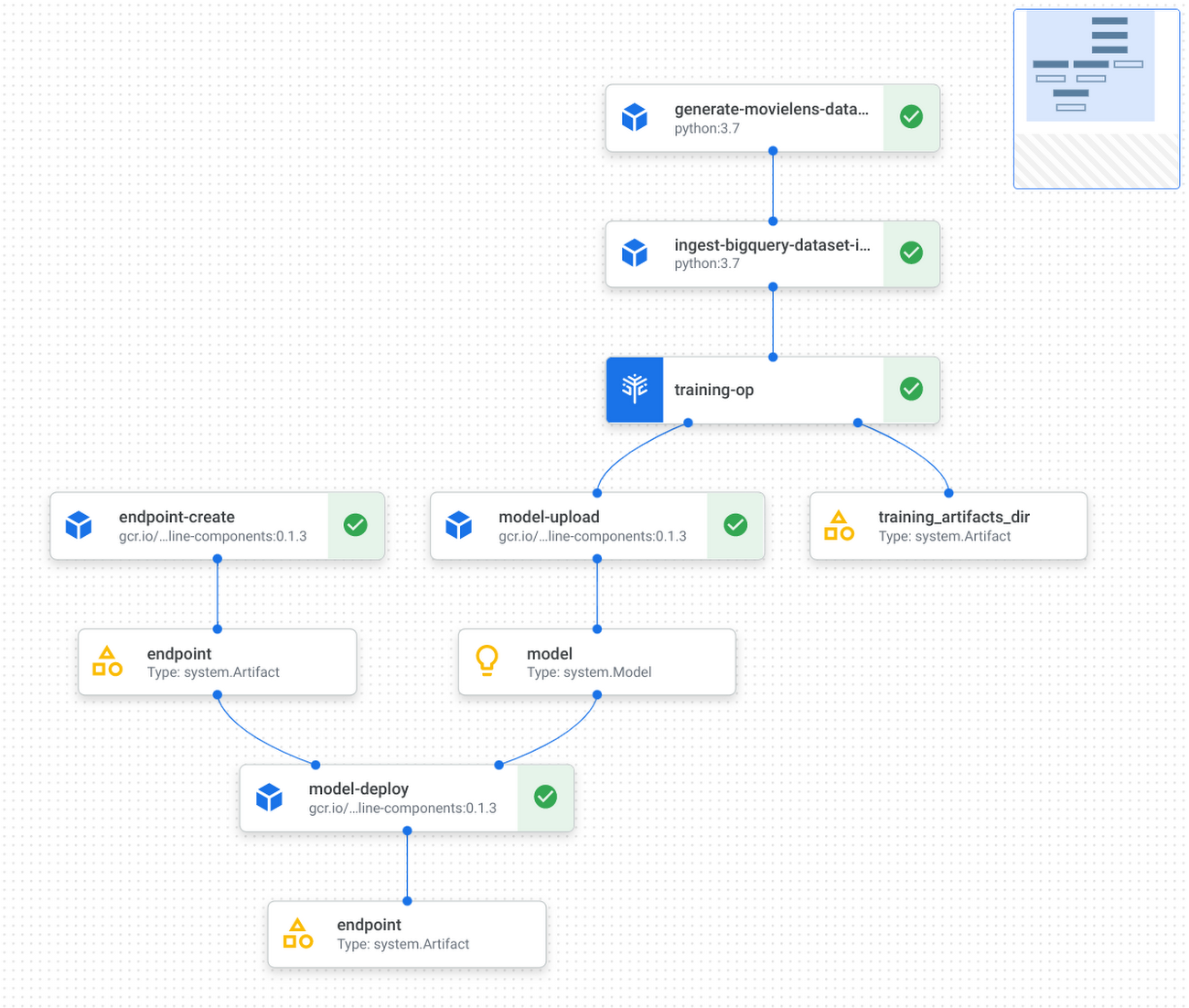
Refer to the GitHub repo for detailed instructions on how to implement and test KFP components, and how to run the pipeline with Vertex Pipelines.
Applying this demo to your own RL projects and production
You can replace the MovieLens simulation environment with a real-world environment where RL quantities like observations, actions and rewards capture relevant aspects of said real-world environment. Based on whether you can interact with the real world in real-time, you may choose either on-policy (showcased by the step-by-step demo) or off-policy (showcased by the pipeline demo) training and evaluation.
If you were to implement a real-world recommendation system, here’s what you’d do:
You would represent users as some user vectors. The individual entries in the user vectors may have actual meanings like age. Alternatively, they may be generated through a neural network as user embeddings. Similarly, you would define what an action is and what actions are possible, likely all items available on your platform; you would also define what the reward is, such as whether the user has tried the item, how long/much the user has spent on the item, user rating of the item, and so on. Again, you have the flexibility to decide on representations for framing the problem that maximize performance. During training or data pre-collection, you may randomly sample users (and build the corresponding user vectors) from the real world, use those vectors as observations to query some policy for items to recommend, and then apply that recommendation to users and obtain their feedback as rewards.
This RL demo can also be extended to ML applications other than recommendation system. For instance, if your use case is to build an image classification system, then you can frame an environment, where observations are the image pixels or embeddings, actions are the predicted classes, and rewards are feedback on the predictions’ correctness.
Conclusion
Congratulations! You have learned how to build reinforcement learning solutions using Vertex AI in a fully managed, modularized and reproducible way. There is so much you can achieve with RL, and you now have many Vertex AI as well as Google Cloud services in your toolbox to support you in your RL endeavors, be it production systems, research or cool personal projects.
Additional resources
- [Recap] step-by-step demo link: GitHub link
- [Recap] end-to-end pipeline demo: GitHub link
- TF-Agents tutorial on bandits: Introduction to Multi-Armed Bandits
- Vertex Pipelines tutorial: Intro to Vertex Pipelines
Unifying Data and AI: Bringing Unstructured Data Analytics to BigQuery

4176
Of your peers have already read this article.
2:30 Minutes
The most insightful time you'll spend today!
Over one third of organizations believe that data analytics and machine learning have the most potential to significantly alter the way they run business over the next 3 to 5 years. However, only 26% of organizations are data driven. One of the biggest reasons for this gap is that a major portion of the data generated today is unstructured, which includes images, documents, and videos. It is estimated to cover roughly up to 80% of all data, which has so far remained untapped by organizations.
One of the goals of Google’s data cloud is to help customers realize value from data of all types and formats. Earlier this year, we announced BigLake, which unifies data lakes and warehouses under a single management framework, enabling you to analyze, search, secure, govern and share unstructured data using BigQuery.
At Next ‘22, we announced the preview of object tables, a new table type in BigQuery that provides a structured record interface for unstructured data stored in Google Cloud Storage. This enables you to directly run analytics and machine learning on images, audio, documents and other file types using existing frameworks like SQL and remote functions natively in BigQuery itself. Object tables also extend our best practices of securing, sharing and governing structured data to unstructured, without needing to learn or deploy new tools.
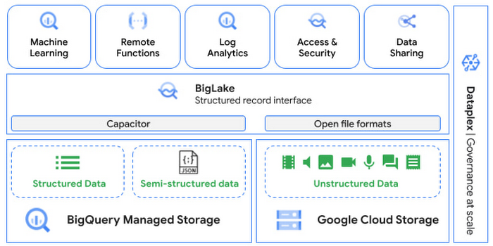
Directly process unstructured data using BigQuery ML
Object tables contain metadata such as URI (Uniform Resource Identifier), content type, and size that can be queried just like other BigQuery tables. You can then derive inferences using machine learning models on unstructured data with BigQuery ML. As part of preview, you can import open source TensorFlow Hub image models, or your own custom models to annotate the images. Very soon, we plan to enable this for audio, video, text and many other formats, and pre-trained models to enable out-of-the box analysis. Check out this video to learn more and watch a demo.
Create an object table
CREATE EXTERNAL TABLE my_dataset.object_table
WITH CONNECTION us.my_connection
OPTIONS(uris=["gs://mybucket/images/*.jpg"],
object_metadata="SIMPLE", metadata_cache_mode="AUTOMATIC");
# Generate inferences with BQML
SELECT * FROM ML.PREDICT(
MODEL my_dataset.vision_model,
(SELECT ML.DECODE_IMAGE(data) AS img FROM my_dataset.object_table)
);By analyzing unstructured data natively in BigQuery, businesses can
- Eliminate manual effort as pre-processing steps such as tuning image sizes to model requirements are automated
- Leverage the simple and familiar SQL interface to quickly gain insights
- Save costs by utilizing existing BigQuery slots without needing to provision new forms of compute
Adswerve is a leading Google Marketing, Analytics and Cloud partner on a mission to humanize data. Twiddy & Co. is Adswerve’s client – a vacation rental company in North Carolina. By combining structured and unstructured data, Twiddy and Adswerve used BigQuery ML to analyze images of rental listings and predict the click-through rate, enabling data-driven photo editorial decisions.
“Twiddy now has the capability to use advanced image analysis to stay competitive in an ever changing landscape of vacation rental providers – and can do this using their in-house SQL skills.” said Pat Grady, Technology Evangelist, Adswerve
Process unstructured data using remote functions
Customers today use remote functions (UDFs) to process structured data for languages and libraries that are not supported in BigQuery. We are extending this capability to process unstructured data using object tables.
Object tables provide signed URLs to allow remote UDFs running on Cloud Functions or Cloud Run to process the object table content. This is particularly useful for running Google’s pre-trained AI models, including Vision AI, Speech-to-Text, Document AI, open source libraries such as Apache Tika, or deploying your own custom models where performance SLAs are important.
Here’s an example of an object table being created over PDF files that are parsed using an open source library running as a remote UDF.
SELECT uri, extract_title(samples.parse_tika(signed_url)) AS title<br>FROM EXTERNAL_OBJECT_TRANSFORM(TABLE pdf_files_object_table,<br>["SIGNED_URL"]);
Extending more BigQuery capabilities to unstructured data
Business intelligence – The results of analyzing unstructured data either directly in BigQuery ML or via UDFs can be combined with your structured data to build unified reports using Looker Studio (at no charge), Looker or any of your preferred BI solutions. This allows you to gain more comprehensive business insights. For example, online retailers can analyze product return rates by correlating them with the images of defective products. Similarly, digital advertisers can correlate ad performance with various attributes of ad creatives to make more informed decisions.
BigQuery search index – Customers are increasingly using the search functionality of BigQuery to power search use cases. These capabilities now extend to unstructured data analytics as well. Whether you use BigQueryML to produce inference on images or use remote UDFs with Doc AI to produce document extraction, the results can now be search indexed and used to support search access patterns.
Here’s an example of search index on data that is parsed from PDF files:
CREATE SEARCH INDEX my_index ON pdf_text_extract(ALL COLUMNS);
SELECT * FROM pdf_text_extract WHERE SEARCH(pdf_text, "Google");Security and governance – We are extending BigQuery’s row-level security capabilities to help you secure objects in Google Cloud Storage. By securing specific rows in an object table, you can restrict the ability of end users to retrieve the signed URLs of corresponding URIs present in the table. This is a shared responsibility security model, for which administrators need to ensure that end users don’t have direct access to Google Cloud Storage, and use signed URLs from object tables as the only access mechanism.
Here’s an example of a policy for PII images that are secured to be first processed through a blur pipeline:
CREATE ROW ACCESS POLICY pii_data ON object_table_images
GRANT TO ("group:admin@example.com")
FILTER USING (ARRAY_LENGTH(metadata)=1 AND
metadata[OFFSET(0)].name="face_detected")
Soon, Dataplex will support object tables, allowing you to automatically create object tables in BigQuery and manage and govern unstructured data at scale.
Data sharing – You can now use Analytics Hub to share unstructured data with partners, customers and suppliers while not compromising on security and governance. Subscribers can consume the rows of object tables that are shared with them, and use signed URLs for unstructured data objects.
Getting Started
Submit this form to try these new capabilities that unlock the power of your unstructured data in BigQuery. Watch this demo to learn more about these new capabilities.
Special thanks to engineering leaders Amir Hormati, Justin Levandoski and Yuri Volobuev for contributing to this post.
More Relevant Stories for Your Company

AI Features in Apigee X Helps Build and Manage APIs at Scale
APIs are the backbone of digital transformation. Via APIs, you can securely share data and functionality with developers both inside and outside of your organizational boundaries, letting you build applications faster, seamlessly connect and interact with partners, and drive new business revenue. Because APIs encompass business-critical information, any downtime or

Geospatial Data for Business Apps Drive Sustainable and Accurate Decision-making
Organizations that collect geospatial data can use that information to understand their operations, help make better business decisions, and power innovation. Traditionally, organizations have required deep GIS expertise and tooling in order to deliver geospatial insights. In this post, we outline some ways that geospatial data can be used in

New Capabilities in BigQuery to Ease Anomalies Detection in the Absence of Labeled Data
When it comes to anomaly detection, one of the key challenges that many organizations face is that it can be difficult to know how to define what an anomaly is. How do you define and anticipate unusual network intrusions, manufacturing defects, or insurance fraud? If you have labeled data with


The Strange Phenomenon AI Revealed at Ride-Hailing Company Go-Jek
Go-Jek, Indonesia’s first billion-dollar startup, has seen an incredible amount of growth in both users and data over the past two years. Many of the ride-hailing company's services are backed by machine learning models hosted on Google Cloud Platform. Models range from driver allocation, to dynamic surge pricing, to food
