User retention can be a major challenge for mobile game developers. According to the Mobile Gaming Industry Analysis in 2019, most mobile games only see a 25% retention rate for users after the first day. To retain a larger percentage of users after their first use of an app, developers can take steps to motivate and incentivize certain users to return. But to do so, developers need to identify the propensity of any specific user returning after the first 24 hours. 

In this blog post, we will discuss how you can use BigQuery ML to run propensity models on Google Analytics 4 data from your gaming app to determine the likelihood of specific users returning to your app.

You can also use the same end-to-end solution approach in other types of apps using Google Analytics for Firebase as well as apps and websites using Google Analytics 4. To try out the steps in this blogpost or to implement the solution for your own data, you can use this Jupyter Notebook. 

Using this blog post and the accompanying Jupyter Notebook, you’ll learn how to:

• Explore the BigQuery export dataset for Google Analytics 4
• Prepare the training data using demographic and behavioural attributes
• Train propensity models using BigQuery ML
• Evaluate BigQuery ML models
• Make predictions using the BigQuery ML models
• Implement model insights in practical implementations

Google Analytics 4 (GA4) properties unify app and website measurement on a single platform and are now default in Google Analytics. Any business that wants to measure their website, app, or both, can use GA4 for a more complete view of how customers engage with their business. With the launch of Google Analytics 4, BigQuery export of Google Analytics data is now available to all users. If you are already using a Google Analytics 4 property, you can follow this guide to set up exporting your GA data to BigQuery.

Once you have set up the BigQuery export, you can explore the data in BigQuery. Google Analytics 4 uses an event-based measurement model. Each row in the data is an event with additional parameters and properties. The Schema for BigQuery Export can help you to understand the structure of the data.  

In this blogpost, we use the public sample export data from an actual mobile game app called “Flood It!” (Android, iOS) to build a churn prediction model. But you can use data from your own app or website. 

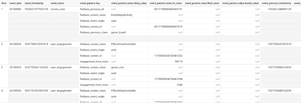
Here’s what the data looks like. Each row in the dataset is a unique event, which can contain nested fields for event parameters.

  SELECT *
FROM `firebase-public-project.analytics_153293282.events_*`
TABLESAMPLE SYSTEM (1 PERCENT)

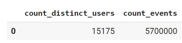
This dataset contains 5.7M events from over 15k users.

  SELECT 
    COUNT(DISTINCT user_pseudo_id) as count_distinct_users,
    COUNT(event_timestamp) as count_events
FROM
  `firebase-public-project.analytics_153293282.events_*

Our goal is to use BigQuery ML on the sample app dataset to predict propensity to user churn or not churn based on users’ demographics and activities within the first 24 hours of app installation.

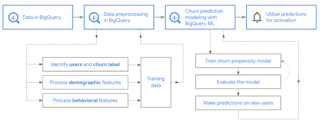
In the following sections, we’ll cover how to:

1. Pre-process the raw event data from GA4
   1. Identify users & the label feature
   2. Process demographic features
   3. Process behavioral features
2. Train classification model using BigQuery ML
3. Evaluate the model using BigQueryML
4. Make predictions using BigQuery ML
5. Utilize predictions for activation

Pre-process the raw event data

You cannot simply use raw event data to train a machine learning model as it would not be in the right shape and format to use as training data. So in this section, we’ll go through how to pre-process the raw data into an appropriate format to use as training data for classification models.

This is what the training data should look like for our use case at the end of this section:

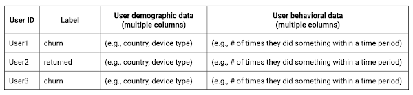
Notice that in this training data, each row represents a unique user with a distinct user ID (user_pseudo_id). 

Identify users & the label feature

We first filtered the dataset to remove users who were unlikely to return the app anyway. We defined these ‘bounced’ users as ones who spent less than 10 mins with the app. Then we labeled all remaining users:

• churned: No event data for the user after 24 hours of first engaging with the app.
• returned: The user has at least one event record after 24 hours of first engaging with the app.

For your use case, you can have a different definition of bounce and churning. Also you can even try to predict something else other than churning, e.g.:

• whether a user is likely to spend money on in-game currency 
• likelihood of completing n-number of game levels
• likelihood of spending n amount of time in-game etc.

In such cases, label each record accordingly so that whatever you are trying to predict can be identified from the label column.

From our dataset, we found that ~41% users (5,557) bounced. However, from the remaining users (8,031),  ~23% (1,883) churned after 24 hours:

  SELECT
    bounced,
    churned, 
    COUNT(churned) as count_users
FROM
    bqmlga4.returningusers
GROUP BY 1,2
ORDER BY bounced

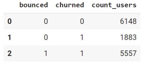
To create these bounced and churned columns, we used the following snippet of SQL code. 

  ...
#churned = 1 if last_touch within 24 hr of app installation, else 0
IF (user_last_engagement < TIMESTAMP_ADD(user_first_engagement, 
      INTERVAL 24 HOUR),
    1,
    0 ) AS churned,
#bounced = 1 if last_touch within 10 min, else 0
IF (user_last_engagement <= TIMESTAMP_ADD(user_first_engagement, 
      INTERVAL 10 MINUTE),
    1,
    0 ) AS bounced,
...

You can view the Jupyter Notebook for the full query used for materializing the bounced and churned labels. 

Process demographic features

Next, we added features both for demographic data and for behavioral data spanning across multiple columns. Having a combination of both demographic data and behavioral data helps to create a more predictive model. 

We used the following fields for each user as demographic features:

• geo.country
• device.operating_system
• device.language

A user might have multiple unique values in these fields — for example if a user uses the app from two different devices. To simplify, we used the values from the very first user engagement event.

  CREATE OR REPLACE VIEW bqmlga4.user_demographics AS (
  WITH first_values AS (
      SELECT
          user_pseudo_id,
          geo.country as country,
          device.operating_system as operating_system,
          device.language as language,
          ROW_NUMBER() OVER (PARTITION BY user_pseudo_id ORDER BY event_timestamp DESC) AS row_num
      FROM `firebase-public-project.analytics_153293282.events_*`
      WHERE event_name="user_engagement"
      )
  SELECT * EXCEPT (row_num)
  FROM first_values
  WHERE row_num = 1 #first engagement
);

Process behavioral features

There is additional demographic information present in the GA4 export dataset, e.g. app_info, device, event_params, geo etc. You may also send demographic information to Google Analytics through each hit via user_properties. Furthermore, if you have first-party data on your own system, you can join that with the GA4 export data based on user_ids. 

To extract user behavior from the data, we looked into the user’s activities within the first 24 hours of first user engagement. In addition to the events automatically collected by Google Analytics, there are also the recommended events for games that can be explored to analyze user behavior. For our use case, to predict user churn, we counted the number of times the follow events were collected for a user within 24 hours of first user engagement: 

• user_engagement
• level_start_quickplay
• level_end_quickplay
• level_complete_quickplay
• level_reset_quickplay
• post_score
• spend_virtual_currency
• ad_reward
• challenge_a_friend
• completed_5_levels
• use_extra_steps

The following query shows how these features were calculated:

  WITH
  events_first24hr AS (
    SELECT
      e.*
    FROM
      `firebase-public-project.analytics_153293282.events_*` e
    JOIN
      bqmlga4.returningusers r
      ON
        e.user_pseudo_id = r.user_pseudo_id
    WHERE
      TIMESTAMP_MICROS(e.event_timestamp) <= r.ts_24hr_after_first_engagement
  )
SELECT
  user_pseudo_id,
  SUM(IF(event_name = 'user_engagement', 1, 0)) AS cnt_user_engagement,
  # ... repeated for all behavior data ... 
  SUM(IF(event_name = 'use_extra_steps', 1, 0)) AS cnt_use_extra_steps,
FROM
  events_first24hr
GROUP BY
  1

View the notebook for the query used to aggregate and extract the behavioral data. You can use different sets of events for your use case. To view the complete list of events, use the following query:

  SELECT
    event_name,
    COUNT(event_name) as event_count
FROM
    `firebase-public-project.analytics_153293282.events_*`
GROUP BY 1
ORDER BY
   event_count DESC

After this we combined the features to ensure our training dataset reflects the intended structure. We had the following columns in our table:

• User ID:
  • user_pseudo_id
• Label:
  • churned
• Demographic features
  • country
  • device_os
  • device_language
• Behavioral features
  • cnt_user_engagement
  • cnt_level_start_quickplay
  • cnt_level_end_quickplay
  • cnt_level_complete_quickplay
  • cnt_level_reset_quickplay
  • cnt_post_score
  • cnt_spend_virtual_currency
  • cnt_ad_reward
  • cnt_challenge_a_friend
  • cnt_completed_5_levels
  • cnt_use_extra_steps
  • user_first_engagement

At this point, the dataset was ready to train the classification machine learning model in BigQuery ML. Once trained, the model will output a propensity score between churn (churned=1) or return (churned=0) indicating the probability of a user churning based on the training data.

Train classification model 

When using the CREATE MODEL statement, BigQuery ML automatically splits the data between training and test. Thus the model can be evaluated immediately after training (see the documentation for more information).

For the ML model, we can choose among the following classification algorithms where each type has its own pros and cons:

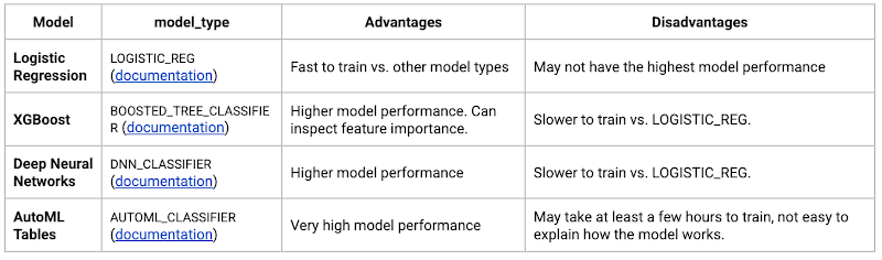
Often logistic regression is used as a starting point because it is the fastest to train. The query below shows how we trained the logistic regression classification models in BigQuery ML.

  CREATE OR REPLACE MODEL bqmlga4.churn_logreg
TRANSFORM(
  EXTRACT(MONTH from user_first_engagement) as month,
  EXTRACT(DAYOFYEAR from user_first_engagement) as julianday,
  EXTRACT(DAYOFWEEK from user_first_engagement) as dayofweek,
  EXTRACT(HOUR from user_first_engagement) as hour,
  * EXCEPT(user_first_engagement, user_pseudo_id)
)
OPTIONS(
  MODEL_TYPE="LOGISTIC_REG",
  INPUT_LABEL_COLS=["churned"]
) AS
SELECT
  *
FROM
  bqmlga4.train

We extracted month, julianday, and dayofweek  from datetimes/timestamps as one simple example of additional feature preprocessing before training. Using TRANSFORM() in your CREATE MODEL query allows the model to remember the extracted values. Thus, when making predictions using the model later on, these values won’t have to be extracted again. View the notebook for the example queries to train other types of models (XGBoost, deep neural network, AutoML Tables).

Evaluate model

Once the model finished training, we ran ML.EVALUATE to generate precision, recall, accuracy and f1_score for the model:

  SELECT
  *
FROM
  ML.EVALUATE(MODEL bqmlga4.churn_logreg)

The optional THRESHOLD parameter can be used to modify the default classification threshold of 0.5. For more information on these metrics, you can read through the definitions on precision and recall, accuracy, f1-score, log_loss and roc_auc. Comparing the resulting evaluation metrics can help to decide among multiple models.Furthermore, we used a confusion matrix to inspect how well the model predicted the labels, compared to the actual labels. The confusion matrix is created using the default threshold of 0.5, which you may want to adjust to optimize for recall, precision, or a balance (more information here).

  SELECT
  expected_label,
  _0 AS predicted_0,
  _1 AS predicted_1
FROM
  ML.CONFUSION_MATRIX(MODEL bqmlga4.churn_logreg)

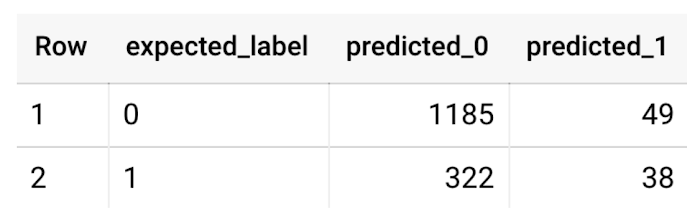
This table can be interpreted in the following way:

Make predictions using BigQuery ML

Once the ideal model was available, we ran ML.PREDICT to make predictions. For propensity modeling, the most important output is the probability of a behavior occurring. The following query returns the probability that the user will return after 24 hrs. The higher the probability and closer it is to 1, the more likely the user is predicted to return, and the closer it is to 0, the more likely the user is predicted to churn.

  SELECT
  user_pseudo_id,
  returned,
  predicted_returned,
  predicted_returned_probs[OFFSET(0)].prob as probability_returned
FROM
  ML.PREDICT(MODEL bqmlga4.churn_logreg,
  (SELECT * FROM bqmlga4.train)) #can be replaced with a proper test dataset

Utilize predictions for activation

Once the model predictions are available for your users, you can activate this insight in different ways. In our analysis, we used user_pseudo_id as the user identifier. However, ideally, your app should send back the user_id from your app to Google Analytics. In addition to using first-party data for model predictions, this will also let you join back the predictions from the model into your own data.

• You can import the model predictions back into Google Analytics as a user attribute. This can be done using the Data Import feature for Google Analytics 4. Based on the prediction values you can Create and edit audiences and also do Audience targeting. For example, an audience can be users with prediction probability between 0.4 and 0.7, to represent users who are predicted to be “on the fence” between churning and returning.
• For Firebase Apps, you can use the Import segments feature. You can tailor user experience by targeting your identified users through Firebase services such as Remote Config, Cloud Messaging, and In-App Messaging. This will involve importing the segment data from BigQuery into Firebase. After that you can send notifications to the users, configure the app for them, or follow the user journeys across devices.
• Run targeted marketing campaigns via CRMs like Salesforce, e.g. send out reminder emails.

You can find all of the code used in this blogpost in the Github repository:

What’s next? 

Continuous model evaluation and re-training

As you collect more data from your users, you may want to regularly evaluate your model on fresh data and re-train the model if you notice that the model quality is decaying.

Continuous evaluation—the process of ensuring a production machine learning model is still performing well on new data—is an essential part in any ML workflow. Performing continuous evaluation can help you catch model drift, a phenomenon that occurs when the data used to train your model no longer reflects the current environment. 

To learn more about how to do continuous model evaluation and re-train models, you can read the blogpost: Continuous model evaluation with BigQuery ML, Stored Procedures, and Cloud Scheduler

More resources

If you’d like to learn more about any of the topics covered in this post, check out these resources:

• BigQuery export of Google Analytics data
• BigQuery ML quickstart
• Events automatically collected by Google Analytics 4
• Qwiklabs: Create ML models with BigQuery ML

Or learn more about how you can use BigQuery ML to easily build other machine learning solutions:

• How to build demand forecasting models with BigQuery ML
• How to build a recommendation system on e-commerce data using BigQuery ML

Let us know what you thought of this post, and if you have topics you’d like to see covered in the future! You can find us on Twitter at @polonglin and @_mkazi_.Thanks to reviewers: Abhishek Kashyap, Breen Baker, David Sabater Dinter.

Cleveland Clinic is one of the largest and most respected hospitals in the United States. Its mission is to provide better care of the sick, investigate their problems, and deliver further education of physicians.

The clinic deployed electronic medical records (EMR) to help doctors deliver greater quality healthcare. But the challenge was, it was not being used at it to its full potential.

“To understand how to use APIs it’s important to understand the challenges that we face. We use the electronic medical record. It’s a great investment we made and it is a great delivery tool but it only gets us so far. For the nurses and the doctors that is not good enough as they are focused in delivering the best possible care,” says Beth Meese, Administrative Director of Technology and Innovations at Cleveland Clinic.

To ensure that the EMR was being used at its full potential the clinic added APIs on top of it.

“Using the Apigee platform, we have been able to write APIs on top of our EMRs and then fill the gap for what the medical records was not able to deliver. APIs help us run analytics, run predictive models, and then surface the data back in a way to the clinicians that they can use to deliver high-quality healthcare,” says Meese.

Leveraging Apigee, Cleveland Clinic was also able to securely give developers access to APIs and reduce a considerable amount of burden from the rest of the IT team.