





3614
Of your peers have already watched this video.
15:20 Minutes
The most insightful time you'll spend today!
Building a Bank with Kubernetes: How Monzo is Creating the Best Banking App Ever
Based in London, Monzo is a bank that lives on the smartphone and is built for the way modern customers live today. By solving their problems, treating them fairly and being totally transparent, Monzo believes it can transform the way people bank.
“We are building a full retail bank. What we are trying to be is become the best banking app in the world. This means that instead of showing you cramped indecipherable descriptors that you get from traditional banks, we actually show you the name of the merchant along with the logo and a real-time balance rather than something that’s often delayed by 24 to 48-hours. Basically, we strive to make everything as clear and easy to understand for customers,” says Oliver Beattie, Head of Engineering, Monzo.
In their quest for building the best banking application, Kubernetes is significantly helping Monzo overcome core banking challenges and continuously innovate.
“Kubernetes makes our application extensible. We want our application to be very easy to change not just now but maybe 10 or 20 years from now. As what we have now will not be the gold standard 20 years down the line. We want our application to be better than those the legacy banks have,” says Beattie.
Running multiple services at the same time on a particular application and ensuring speed was a significant hurdle Monzo had to overcome.
“You cannot run 150 services on a single machine and expect all of them to be fast. What we wanted is to treat our application as a big pool of resources, which is what Kubernetes exactly allowed us to do. We can now run one big group of worker machines and run all our applications there and scale them up and down as needed. Owing to Kubernetes we are now able to reduce one-third of our infrastructure costs,” says Beattie.
Watch the full video to get deeper insights into how Kubernetes is helping Monzo build the best banking application ever.
3217
Of your peers have already watched this video.
2:00 Minutes
The most insightful time you'll spend today!
Simplified Document Processing with AppSheet Automation
Move over legacy, time-consuming systems and processes to update data from documents and invoices into disparate data systems. AppSheet integrates no-code development with Google Cloud’s state-of-the-art Document AI to automate the data extraction and validation from invoices, documents, receipts, etc.
You can end all ‘guesstimates’ and rely on the accuracy of the intelligent document processing feature, and set custom triggers for automation events or the way data is displayed from its unstructured source. Watch the video to understand how your business can save time and resources with automation and seamlessly manage high-volume, unstructured data.
Scaling with Breaking News: BBC’s Serverless Infrastructure on Google Cloud

1264
Of your peers have already read this article.
3:30 Minutes
The most insightful time you'll spend today!
Editors note: Today’s post is from Neil Craig at the British Broadcasting Corporation (BBC), the national broadcaster of the United Kingdom. Neil is part of the BBC’s Digital Distribution team which is responsible for building the services such as the public-facing www bbc.co.uk and .com websites and ensuring they are able to scale and operate reliably.
The BBC’s public-facing websites inform, educate, and entertain over 498 million adults per week across the world. Because breaking news is so unpredictable, we need a core content delivery platform that can easily scale in response to surges in traffic, which can be quite unpredictable.
To this end, we recently rebuilt our log-processing infrastructure on a Google Cloud serverless platform. We’ve found that the new system, based on Cloud Storage, Eventarc, Cloud Run and BigQuery, enables us to provide a reliable and stable service without us having to worry about scaling up during busy times. We’re also able to save license fee payers money by operating the service more cost effectively than our previous architecture. Not having to manually manage the scale of major components of the stack has freed up our time, allowing us to spend it on using, rather than creating the data.
A log in time
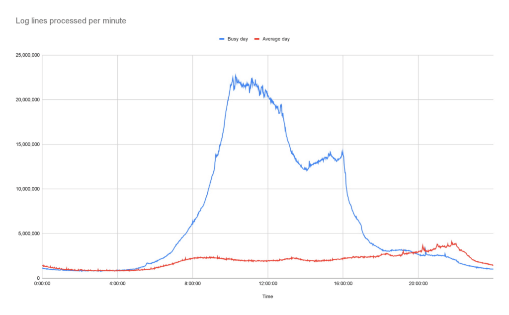
To operate the site and ensure our services run smoothly we continually monitor Traffic Manager and CDN access logs. Our websites generate more than 3B log lines per day, and handle large data bursts during major news events; on a busy day our system supports over 26B log lines in a single day.
As initially designed, we stored log data in a Cloud Storage bucket. But every time we needed to access that data, we had to download terabytes of logs down to a virtual machine (VM) with a large amount of attached storage, and use the ‘grep’ tool to search and analyze them. From beginning to end, this took us several hours. On heavy news days, the time lag made it difficult for the engineering team to do their jobs.
We needed a more efficient way to make this log data available, so we designed and deployed a new system that deals with logs and reacts to spikes more efficiently as they arrive, improving the timeliness of critical information significantly.
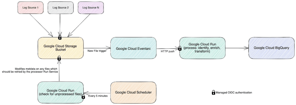
In this new system, we still leverage Cloud Storage buckets, but on arrival, each log generates an event using EventArc. That event triggers Cloud Run to validate, transform and enrich various pieces of information about the log file such as filename, prefix, and type, then processes it and outputs the processed data as a stream into BigQuery. This event-driven design allows us to process files quickly and frequently — processing a single log file typically takes less than a second. Most of the files that we feed into the system are small, fewer than 100 Megabytes, but for larger files, we automatically split those into multiple files and Cloud Run automatically creates additional parallel instances very quickly, helping the system scale almost instantly.
The nature of running a global website which provides news coverage means we see frequent, unpredictable large spikes of traffic. We learn from these and optimize our systems where necessary so we’re confident in the system’s ability to handle significant traffic. For example, around the time of the announcement of the Queen’s passing in September, we saw some huge traffic spikes. During the largest, within one minute, we went from running 150 – 200 container instances to over 1000…. and the infrastructure just worked. Because we engineered the log processing system to rely on the elasticity of a serverless architecture, we knew from the get-go that it would be able to handle this type of scaling.
Around the time of the announcement of the Queen’s passing in September, we saw some huge traffic spikes. During the largest, within one minute, we went from running 150 – 200 container instances to over 1000…. and the infrastructure just worked
Our initial concern about choosing serverless was cost. It turns out that using Cloud Run is significantly more cost-effective than running the number of VMs we would need for a system that could survive reasonable traffic spikes with a similar level of confidence.
Switching to Cloud Run also allows us to use our time more efficiently, as we no longer need to spend time managing and monitoring VM scaling or resource usage. We picked Cloud Run intentionally because we wanted a system that could scale well without manual intervention. As the digital distribution team, our job is not to do ops work on the underlying components of this system — we leave that to the specialist ops teams at Google.
Another conscious choice we made whilst rebuilding the system was to use the built-in service-to-service authentication in Google Cloud. Rather than implementing and maintaining the authentication mechanism ourselves, we add some simple configuration which instructs the client side to create and send a OIDC token for a service account we define and the server side to authenticate and authorize the client. Another example is pushing events into Cloud Run, where we can configure Cloud Run authorization to only accept events from specific EventArc triggers, so it is fully private.
Going forward, the new system has allowed us to make better use of our data safely. For example, BigQuery’s per-column permissions allow us to open up access to our logs to other engineering teams around the organization, without having to worry about sharing PII that’s restricted to approved users.
The goal of our team is to empower all teams within the BBC to get the content they want on the web when they want it, make it reliable, secure, and make sure it can scale. Google Cloud serverless products helped us to achieve these goals with relatively little effort and require significantly less management than previous generations of technology.
3380
Of your peers have already watched this video.
19:00 Minutes
The most insightful time you'll spend today!
Booking.com’s Apigee Hybrid on Anthos is the Largest Hybrid Deployment Ever
Apigee API Management Platform helps unlock the value of data in legacy systems and applications to accelerate end-user/customer experience by modernizing apps and building multi-cloud environments. With Apigee Hybrid on Anthos, a service mesh technology, Booking.com was able to achieve its goal of providing customers a connected trip experience. Watch the video to understand how Booking.com, a biggest brand in Booking Holdings portfolio with over 1.5 million room bookings in 24 hours moved to hybrid cloud and unified APIs to one platform offering a end-to-end customer journey for a connected trip!
10135
Of your peers have already watched this video.
1:00 Minutes
The most insightful time you'll spend today!
Predict User Churn on Gaming Apps with Google Analytics Data using BigQuery ML
User retention can be a major challenge for mobile game developers. According to the Mobile Gaming Industry Analysis in 2019, most mobile games only see a 25% retention rate for users after the first day. To retain a larger percentage of users after their first use of an app, developers can take steps to motivate and incentivize certain users to return. But to do so, developers need to identify the propensity of any specific user returning after the first 24 hours.
In this blog post, we will discuss how you can use BigQuery ML to run propensity models on Google Analytics 4 data from your gaming app to determine the likelihood of specific users returning to your app.
You can also use the same end-to-end solution approach in other types of apps using Google Analytics for Firebase as well as apps and websites using Google Analytics 4. To try out the steps in this blogpost or to implement the solution for your own data, you can use this Jupyter Notebook.
Using this blog post and the accompanying Jupyter Notebook, you’ll learn how to:
- Explore the BigQuery export dataset for Google Analytics 4
- Prepare the training data using demographic and behavioural attributes
- Train propensity models using BigQuery ML
- Evaluate BigQuery ML models
- Make predictions using the BigQuery ML models
- Implement model insights in practical implementations
Google Analytics 4 (GA4) properties unify app and website measurement on a single platform and are now default in Google Analytics. Any business that wants to measure their website, app, or both, can use GA4 for a more complete view of how customers engage with their business. With the launch of Google Analytics 4, BigQuery export of Google Analytics data is now available to all users. If you are already using a Google Analytics 4 property, you can follow this guide to set up exporting your GA data to BigQuery.
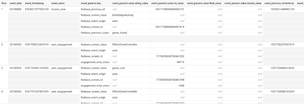
Once you have set up the BigQuery export, you can explore the data in BigQuery. Google Analytics 4 uses an event-based measurement model. Each row in the data is an event with additional parameters and properties. The Schema for BigQuery Export can help you to understand the structure of the data.
In this blogpost, we use the public sample export data from an actual mobile game app called “Flood It!” (Android, iOS) to build a churn prediction model. But you can use data from your own app or website.
Here’s what the data looks like. Each row in the dataset is a unique event, which can contain nested fields for event parameters.
SELECT *FROM `firebase-public-project.analytics_153293282.events_*`TABLESAMPLE SYSTEM (1 PERCENT)
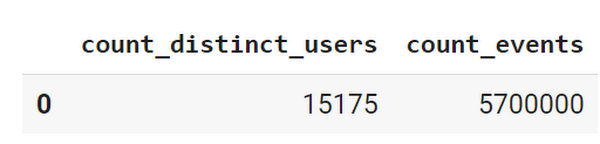
This dataset contains 5.7M events from over 15k users.
SELECTCOUNT(DISTINCT user_pseudo_id) as count_distinct_users,COUNT(event_timestamp) as count_eventsFROM`firebase-public-project.analytics_153293282.events_*
Our goal is to use BigQuery ML on the sample app dataset to predict propensity to user churn or not churn based on users’ demographics and activities within the first 24 hours of app installation.
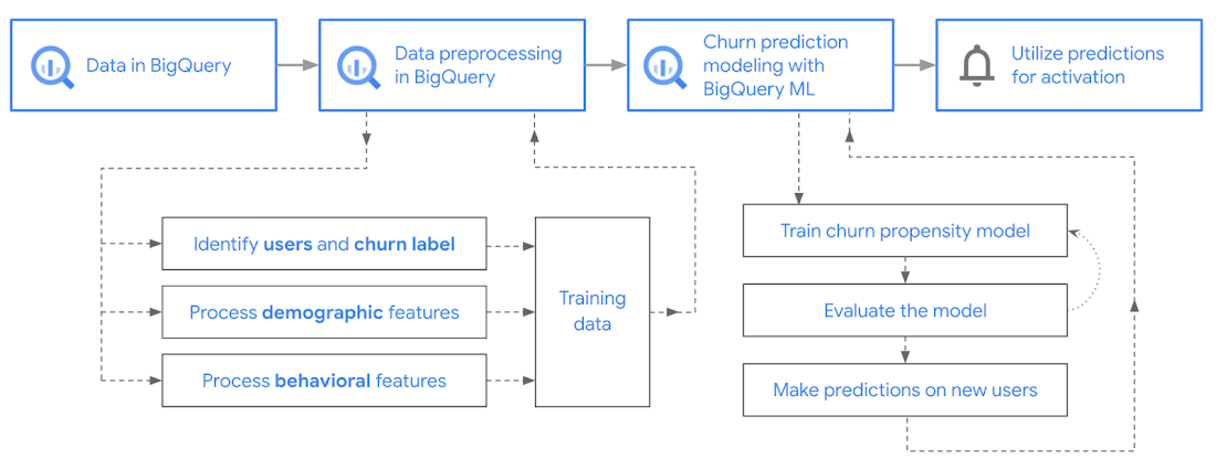
In the following sections, we’ll cover how to:
- Pre-process the raw event data from GA4
- Identify users & the label feature
- Process demographic features
- Process behavioral features
- Train classification model using BigQuery ML
- Evaluate the model using BigQueryML
- Make predictions using BigQuery ML
- Utilize predictions for activation
Pre-process the raw event data
You cannot simply use raw event data to train a machine learning model as it would not be in the right shape and format to use as training data. So in this section, we’ll go through how to pre-process the raw data into an appropriate format to use as training data for classification models.
This is what the training data should look like for our use case at the end of this section:
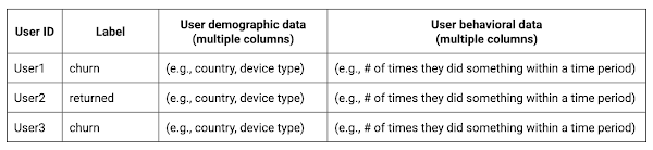
Notice that in this training data, each row represents a unique user with a distinct user ID (user_pseudo_id).
Identify users & the label feature
We first filtered the dataset to remove users who were unlikely to return the app anyway. We defined these ‘bounced’ users as ones who spent less than 10 mins with the app. Then we labeled all remaining users:
- churned: No event data for the user after 24 hours of first engaging with the app.
- returned: The user has at least one event record after 24 hours of first engaging with the app.
For your use case, you can have a different definition of bounce and churning. Also you can even try to predict something else other than churning, e.g.:
- whether a user is likely to spend money on in-game currency
- likelihood of completing n-number of game levels
- likelihood of spending n amount of time in-game etc.
In such cases, label each record accordingly so that whatever you are trying to predict can be identified from the label column.
From our dataset, we found that ~41% users (5,557) bounced. However, from the remaining users (8,031), ~23% (1,883) churned after 24 hours:
SELECTbounced,churned,COUNT(churned) as count_usersFROMbqmlga4.returningusersGROUP BY 1,2ORDER BY bounced
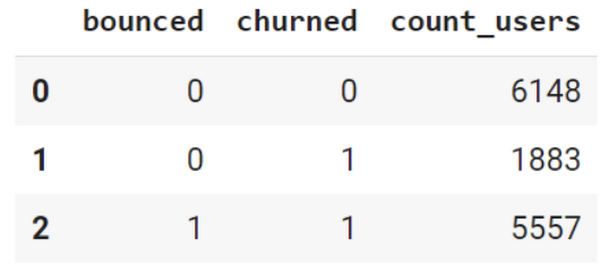
To create these bounced and churned columns, we used the following snippet of SQL code.
...#churned = 1 if last_touch within 24 hr of app installation, else 0IF (user_last_engagement < TIMESTAMP_ADD(user_first_engagement,INTERVAL 24 HOUR),1,0 ) AS churned,#bounced = 1 if last_touch within 10 min, else 0IF (user_last_engagement <= TIMESTAMP_ADD(user_first_engagement,INTERVAL 10 MINUTE),1,0 ) AS bounced,...
You can view the Jupyter Notebook for the full query used for materializing the bounced and churned labels.
Process demographic features
Next, we added features both for demographic data and for behavioral data spanning across multiple columns. Having a combination of both demographic data and behavioral data helps to create a more predictive model.
We used the following fields for each user as demographic features:
geo.countrydevice.operating_systemdevice.language
A user might have multiple unique values in these fields — for example if a user uses the app from two different devices. To simplify, we used the values from the very first user engagement event.
CREATE OR REPLACE VIEW bqmlga4.user_demographics AS (WITH first_values AS (SELECTuser_pseudo_id,geo.country as country,device.operating_system as operating_system,device.language as language,ROW_NUMBER() OVER (PARTITION BY user_pseudo_id ORDER BY event_timestamp DESC) AS row_numFROM `firebase-public-project.analytics_153293282.events_*`WHERE event_name="user_engagement")SELECT * EXCEPT (row_num)FROM first_valuesWHERE row_num = 1 #first engagement);
Process behavioral features
There is additional demographic information present in the GA4 export dataset, e.g. app_info, device, event_params, geo etc. You may also send demographic information to Google Analytics through each hit via user_properties. Furthermore, if you have first-party data on your own system, you can join that with the GA4 export data based on user_ids.
To extract user behavior from the data, we looked into the user’s activities within the first 24 hours of first user engagement. In addition to the events automatically collected by Google Analytics, there are also the recommended events for games that can be explored to analyze user behavior. For our use case, to predict user churn, we counted the number of times the follow events were collected for a user within 24 hours of first user engagement:
user_engagementlevel_start_quickplaylevel_end_quickplaylevel_complete_quickplaylevel_reset_quickplaypost_scorespend_virtual_currencyad_rewardchallenge_a_friendcompleted_5_levelsuse_extra_steps
The following query shows how these features were calculated:
WITHevents_first24hr AS (SELECTe.*FROM`firebase-public-project.analytics_153293282.events_*` eJOINbqmlga4.returningusers rONe.user_pseudo_id = r.user_pseudo_idWHERETIMESTAMP_MICROS(e.event_timestamp) <= r.ts_24hr_after_first_engagement)SELECTuser_pseudo_id,SUM(IF(event_name = 'user_engagement', 1, 0)) AS cnt_user_engagement,# ... repeated for all behavior data ...SUM(IF(event_name = 'use_extra_steps', 1, 0)) AS cnt_use_extra_steps,FROMevents_first24hrGROUP BY1
View the notebook for the query used to aggregate and extract the behavioral data. You can use different sets of events for your use case. To view the complete list of events, use the following query:
SELECTevent_name,COUNT(event_name) as event_countFROM`firebase-public-project.analytics_153293282.events_*`GROUP BY 1ORDER BYevent_count DESC
After this we combined the features to ensure our training dataset reflects the intended structure. We had the following columns in our table:
- User ID:
user_pseudo_id
- Label:
churned
- Demographic features
countrydevice_osdevice_language
- Behavioral features
cnt_user_engagementcnt_level_start_quickplaycnt_level_end_quickplaycnt_level_complete_quickplaycnt_level_reset_quickplaycnt_post_scorecnt_spend_virtual_currencycnt_ad_rewardcnt_challenge_a_friendcnt_completed_5_levelscnt_use_extra_stepsuser_first_engagement
At this point, the dataset was ready to train the classification machine learning model in BigQuery ML. Once trained, the model will output a propensity score between churn (churned=1) or return (churned=0) indicating the probability of a user churning based on the training data.
Train classification model
When using the CREATE MODEL statement, BigQuery ML automatically splits the data between training and test. Thus the model can be evaluated immediately after training (see the documentation for more information).
For the ML model, we can choose among the following classification algorithms where each type has its own pros and cons:
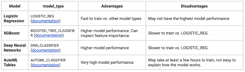
Often logistic regression is used as a starting point because it is the fastest to train. The query below shows how we trained the logistic regression classification models in BigQuery ML.
CREATE OR REPLACE MODEL bqmlga4.churn_logregTRANSFORM(EXTRACT(MONTH from user_first_engagement) as month,EXTRACT(DAYOFYEAR from user_first_engagement) as julianday,EXTRACT(DAYOFWEEK from user_first_engagement) as dayofweek,EXTRACT(HOUR from user_first_engagement) as hour,* EXCEPT(user_first_engagement, user_pseudo_id))OPTIONS(MODEL_TYPE="LOGISTIC_REG",INPUT_LABEL_COLS=["churned"]) ASSELECT*FROMbqmlga4.train
We extracted month, julianday, and dayofweek from datetimes/timestamps as one simple example of additional feature preprocessing before training. Using TRANSFORM() in your CREATE MODEL query allows the model to remember the extracted values. Thus, when making predictions using the model later on, these values won’t have to be extracted again. View the notebook for the example queries to train other types of models (XGBoost, deep neural network, AutoML Tables).
Evaluate model
Once the model finished training, we ran ML.EVALUATE to generate precision, recall, accuracy and f1_score for the model:
SELECT*FROMML.EVALUATE(MODEL bqmlga4.churn_logreg)

The optional THRESHOLD parameter can be used to modify the default classification threshold of 0.5. For more information on these metrics, you can read through the definitions on precision and recall, accuracy, f1-score, log_loss and roc_auc. Comparing the resulting evaluation metrics can help to decide among multiple models.Furthermore, we used a confusion matrix to inspect how well the model predicted the labels, compared to the actual labels. The confusion matrix is created using the default threshold of 0.5, which you may want to adjust to optimize for recall, precision, or a balance (more information here).
SELECTexpected_label,_0 AS predicted_0,_1 AS predicted_1FROMML.CONFUSION_MATRIX(MODEL bqmlga4.churn_logreg)
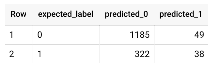
This table can be interpreted in the following way:

Make predictions using BigQuery ML
Once the ideal model was available, we ran ML.PREDICT to make predictions. For propensity modeling, the most important output is the probability of a behavior occurring. The following query returns the probability that the user will return after 24 hrs. The higher the probability and closer it is to 1, the more likely the user is predicted to return, and the closer it is to 0, the more likely the user is predicted to churn.
SELECTuser_pseudo_id,returned,predicted_returned,predicted_returned_probs[OFFSET(0)].prob as probability_returnedFROMML.PREDICT(MODEL bqmlga4.churn_logreg,(SELECT * FROM bqmlga4.train)) #can be replaced with a proper test dataset
Utilize predictions for activation
Once the model predictions are available for your users, you can activate this insight in different ways. In our analysis, we used user_pseudo_id as the user identifier. However, ideally, your app should send back the user_id from your app to Google Analytics. In addition to using first-party data for model predictions, this will also let you join back the predictions from the model into your own data.
- You can import the model predictions back into Google Analytics as a user attribute. This can be done using the Data Import feature for Google Analytics 4. Based on the prediction values you can Create and edit audiences and also do Audience targeting. For example, an audience can be users with prediction probability between 0.4 and 0.7, to represent users who are predicted to be “on the fence” between churning and returning.
- For Firebase Apps, you can use the Import segments feature. You can tailor user experience by targeting your identified users through Firebase services such as Remote Config, Cloud Messaging, and In-App Messaging. This will involve importing the segment data from BigQuery into Firebase. After that you can send notifications to the users, configure the app for them, or follow the user journeys across devices.
- Run targeted marketing campaigns via CRMs like Salesforce, e.g. send out reminder emails.
You can find all of the code used in this blogpost in the Github repository:
What’s next?
Continuous model evaluation and re-training
As you collect more data from your users, you may want to regularly evaluate your model on fresh data and re-train the model if you notice that the model quality is decaying.
Continuous evaluation—the process of ensuring a production machine learning model is still performing well on new data—is an essential part in any ML workflow. Performing continuous evaluation can help you catch model drift, a phenomenon that occurs when the data used to train your model no longer reflects the current environment.
To learn more about how to do continuous model evaluation and re-train models, you can read the blogpost: Continuous model evaluation with BigQuery ML, Stored Procedures, and Cloud Scheduler
More resources
If you’d like to learn more about any of the topics covered in this post, check out these resources:
- BigQuery export of Google Analytics data
- BigQuery ML quickstart
- Events automatically collected by Google Analytics 4
- Qwiklabs: Create ML models with BigQuery ML
Or learn more about how you can use BigQuery ML to easily build other machine learning solutions:
- How to build demand forecasting models with BigQuery ML
- How to build a recommendation system on e-commerce data using BigQuery ML
Let us know what you thought of this post, and if you have topics you’d like to see covered in the future! You can find us on Twitter at @polonglin and @_mkazi_.Thanks to reviewers: Abhishek Kashyap, Breen Baker, David Sabater Dinter.
Google Maps’ Cloud-based Styling Features Betters UX, Control and Flexibility

3356
Of your peers have already read this article.
2:00 Minutes
The most insightful time you'll spend today!
This year at Google I/O, we announced the general availability of Cloud-based maps styling for the Maps JavaScript API. In an effort to provide you with more options and more control to help create the best experience for your users, today we’re releasing new features to Cloud-based maps styling. You may already be familiar with these features from the consumer Google Maps web and mobile apps—Landmarks and Building Footprints. We’re also releasing updates to our industry optimized map styles to provide even more map details while providing the flexibility to craft the best experience for your users. Let’s take a look.
Help users quickly scan and orient themselves with Landmarks
You may have noticed some enhancements for prominent places in the consumer Google Maps web and mobile apps, these landmarks help show your users points of interest that help them orient and navigate cities they are exploring or visiting.
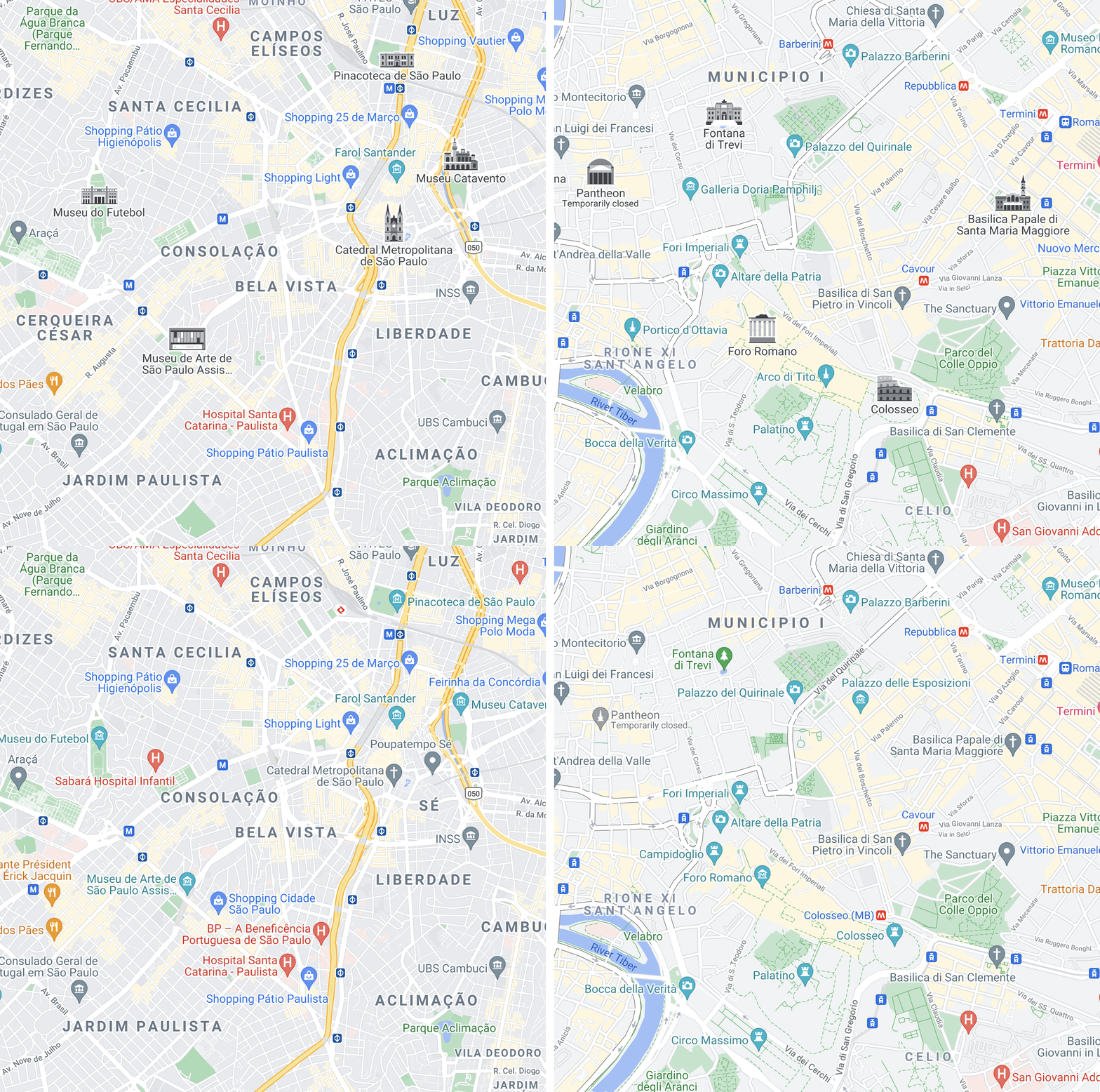
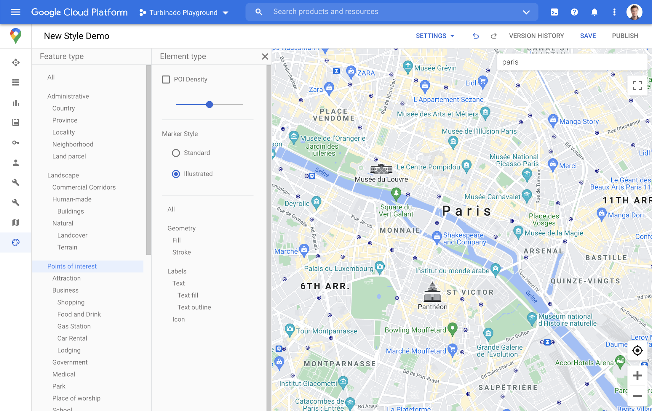
You now have the ability to bring this same experience to your users by creating maps using Cloud-based maps styling. This feature is available in 100 cities globally including New York, Dubai, Paris, Mumbai, and Singapore. To enable landmarks for your map, log into the Cloud console and in our style editor navigate to the Points of interest feature type and select ‘Illustrated’ under Marker Style.
Simplify maps features by switching to Building Footprints
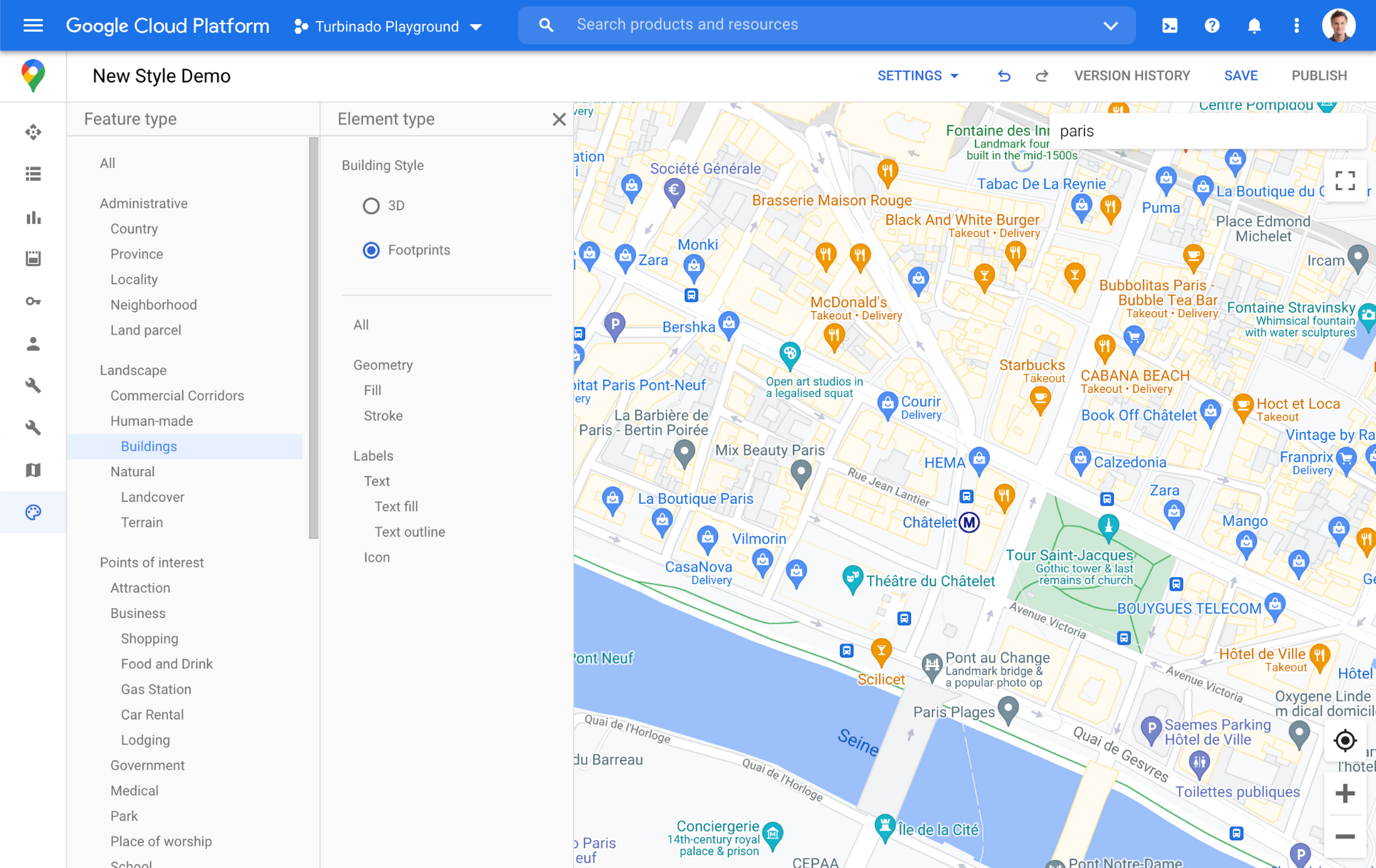
Sometimes less is more. In dense, highly vertical cities, showing 3D building heights can add cognitive load for users. Now, in addition to 3D buildings, we offer building footprints as an option in the style editor. Building footprints can provide a strikingly different basemap balance and composition to better support use cases that may not benefit from the added complexity that 3D buildings can present.

Fill and stroke geometries can also be styled independently to support various color themes. To enable Building Footprints, log into the Cloud console and in our style editor navigate to Buildings and choose ‘Footprints’ under building style.
Industry Optimized Map Styles now include Landmarks and Building Footprints, plus Detailed Street Maps
In January of this year we launched Industry Optimized Map Styles for the travel, real estate, retail, and logistics industries, providing customers with pre-styled map configurations, available via Cloud-based maps styling. Landmarks are now included in all of our Industry Optimized Map Styles and we have turned on Building Footprints in the travel style map. If you are already an Industry Optimized Map Styles user, these new features will be applied to your map with no action needed from you. If you would like to disable these changes, you can use the style editor to turn off these features.
For Industry Optimized Map Styles only, we are also excited to enable Detailed Street Maps. You may have seen these features in our consumer products at Google I/O, released back in August of 2020 for the consumer Google Maps web and mobile apps. Detailed Street Maps are available in San Francisco, New York, London, and Tokyo, and we are targeting expansion to 50 new cities by the end of 2021.
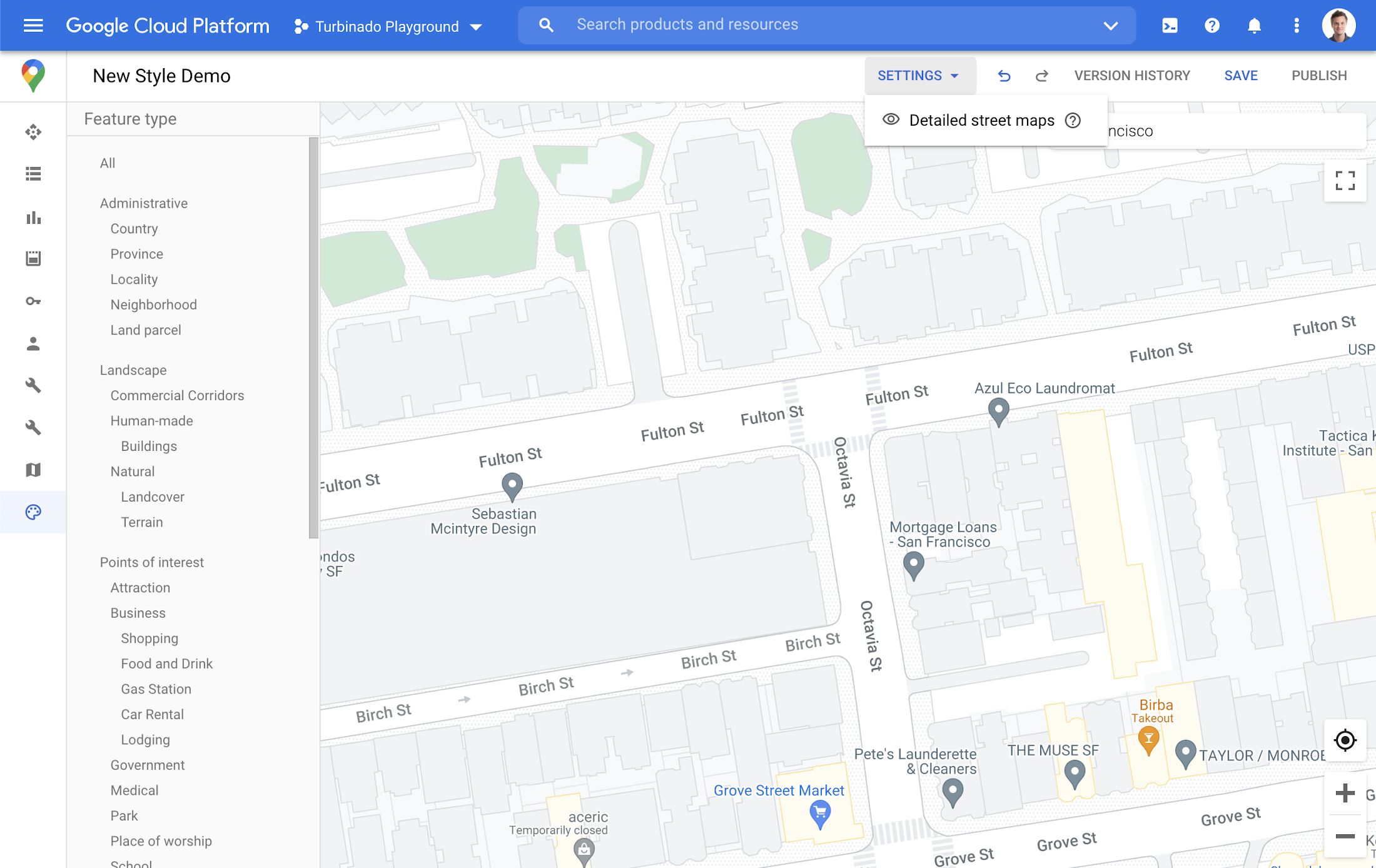
Detailed Street Maps are on by default for all Industry Optimized Map Styles and we created a new settings menu to change the visibility, as needed. We are working on bringing the full styling capability for Detailed Street Maps features to all Cloud-based maps styles in the future.
Landmarks and Building Footprints as well as the updates to Industry Optimized Map Styles are only available via Cloud-based map styling in the Google Cloud Console and are included in Google Maps Platform pricing. Learn more about how to use Landmarks and Building Footprints and Industry Optimized Map Styles. To get started with Cloud-based map styling, check out our documentation for JavaScript.
For more information on Google Maps Platform, visit our website.
More Relevant Stories for Your Company

How Smart Parking Transformed into a Data-Intelligent Business
Google Cloud Results Reduced smart parking/smart city IoT installation and operational support effort by more than halfEnabled development of a Smart Cloud IoT platform in just four monthsDemocratised data access and use across the organisationBuilt core infrastructure in under 4 months Smart Parking’s core product is a sensor-based system called

Conquering Hybrid API Management: Building The Perfect Team and Platform
Introduction In our discussions with technology leaders from around the world for – The Digital Crunch Time: 2022 State of APIs and Applications – two themes emerged #1 Cloud — and hybrid cloud specifically — is becoming a driving factor of success with 59% of respondents saying they were looking to increase

Artifact Registry: An Extension Capabilities of Container Registry
Enterprise application teams need to manage more than just containers in their software supply chain. That’s why we created Artifact Registry, a fully-managed service with support for both container images and non-container artifacts. Artifact Registry improves and extends upon the existing capabilities of Container Registry, such as customer-managed encryption keys, VPC-SC support,

Three Reasons Why Enterprises Must Think Next-gen Serverless
As we reflect on the past year, Heraclitus' phrase “The only constant in life is change” has never rang more true. With the pandemic, companies had to shift operations, launch new products and adapt to extreme demand patterns, sometimes within a matter of weeks. To respond to customer needs faster
