





New ML-Powered API Abuse Detection

1577
Of your peers have already read this article.
3:30 Minutes
The most insightful time you'll spend today!
API security incidents are increasingly common and disruptive. With the growth of API traffic, enterprises across the world are also experiencing an uptick in malicious API attacks, making API security a heightened priority. According to our latest API Security Research Report, 50% of organizations surveyed have experienced an API security incident in the past 12 months and of those, 77% delayed the rollout of a new service or application.
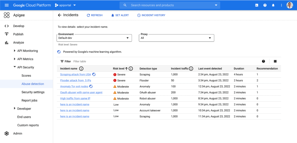
At the RSA Conference 2023 today, we’re making it faster and easier to help detect API abuse incidents with the introduction of Advanced API Security Machine Learning powered abuse-detection dashboards. Our newly introduced Machine Learning models are trained to detect business logic attacks.
These types of attacks are notoriously hard to identify, and target APIs tied to intellectual property, business processes, or sensitive information, such as user data, listing of goods, or crediting accounts. These APIs must be accessible to provide business value, but have also become targets for attackers.
API security incidents can have a considerable impact on an organization’s operations and its bottom line. In June 2022, Imperva released a report titled Quantifying the Cost of API Insecurity, which estimates that lack of secure APIs could result in an average annual API-related total global cyber loss of between $41 billion to $75 billion annually. Furthermore, according to IBM’s 2022 Cost of a Data Breach Report, the average cost of a data breach is $4.35 million. It’s vital that organizations detect and mitigate API abuse incidents early to prevent prolonged fiscal and reputational damage to the business.
However, business logic attacks are harder to detect using static security policies, which allows attackers to manipulate legitimate functionality to achieve a malicious goal without triggering any static security alerts. For example, if a malicious actor gains control of a server and makes subtle changes, the shift in activity patterns of the server is generally undetectable to most monitoring tools. However, in this scenario, the Advanced API Security’s ML-powered API abuse detection model can help differentiate between legitimate and deviant traffic and immediately notify key stakeholders to act quickly and minimize blast radius of the problem.
The ML models that power API abuse detection have been trained and used by Google’s internal teams to help protect our public-facing APIs. The models rely on years of learning and best practices and are now available to all Apigee Advanced API Security customers.
Another challenge in detecting API abuse incidents is the volume of alerts. To reduce the risk of missing key security incidents, many static rules that detect less sophisticated attacks are incredibly sensitive: They generate a high volume of alerts. This makes finding the critical incidents within API traffic and acting to resolve them like “finding a needle in a haystack” for many IT teams. Apigee Advanced Security’s ML-powered dashboards more accurately identify critical API abuses and find similar patterns within the large number of bot alerts to help reduce the time to find and act on most important incidents.
With the help of Apigee Advanced API Security’s ML-powered abuse detection dashboards, customers can uncover critical API abuse incidents, including business logic attacks, scraping, and anomalies, faster. Critical threats are surfaced with clear and concise descriptions to capture the essence of the attack along with the most important characteristics such as the source of the attack, the number of API calls, and the duration of the attack, to help resolve the incident more rapidly.
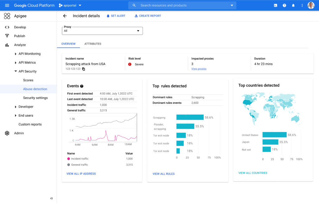
Machine Learning powered abuse-detection dashboards are available in Advanced API Security, a feature of Apigee API management that enables you to more easily detect API security misconfigurations, bad bots, and malicious activities.
To get started with Advanced API Security’s ML-powered dashboards, start your free Apigee trial now.
New Capabilities in BigQuery to Ease Anomalies Detection in the Absence of Labeled Data

6331
Of your peers have already read this article.
4:00 Minutes
The most insightful time you'll spend today!
When it comes to anomaly detection, one of the key challenges that many organizations face is that it can be difficult to know how to define what an anomaly is. How do you define and anticipate unusual network intrusions, manufacturing defects, or insurance fraud? If you have labeled data with known anomalies, then you can choose from a variety of supervised machine learning model types that are already supported in BigQuery ML. But what can you do if you don’t know what kind of anomaly to expect, and you don’t have labeled data? Unlike typical predictive techniques that leverage supervised learning, organizations may need to be able to detect anomalies in the absence of labeled data.
Today we are announcing the public preview of new anomaly detection capabilities in BigQuery ML that leverage unsupervised machine learning to help you detect anomalies without needing labeled data. Depending on whether or not the training data is time series, users can now detect anomalies in training data or on new input data using a new ML.DETECT_ANOMALIES function (documentation), with the following models:
- Autoencoder model, now in Public Preview (documentation)
- K-means model, already GA (documentation)
- ARIMA_PLUS time series model, already GA (documentation)
How does anomaly detection with ML.DETECT_ANOMALIES work?
To detect anomalies in non-time-series data, you can use:
- K-means clustering models: When you use
ML.DETECT_ANOMALIESwith a k-means model, anomalies are identified based on the value of each input data point’s normalized distance to its nearest cluster. If that distance exceeds a threshold determined by the contamination value provided by the user, the data point is identified as an anomaly. - Autoencoder models: When you use
ML.DETECT_ANOMALIESwith an autoencoder model, anomalies are identified based on the reconstruction error for each data point. If the error exceeds a threshold determined by the contamination value, it is identified as an anomaly.
To detect anomalies in time-series data, you can use:
- ARIMA_PLUS time series models: When you use
ML.DETECT_ANOMALIESwith an ARIMA_PLUS model, anomalies are identified based on the confidence interval for that timestamp. If the probability that the data point at that timestamp occurs outside of the prediction interval exceeds a probability threshold provided by the user, the datapoint is identified as an anomaly.
Below we show code examples of anomaly detection in BigQuery ML for each of the above scenarios.
Anomaly detection with a k-means clustering model
You can now detect anomalies using k-means clustering models, by running ML.DETECT_ANOMALIES to detect anomalies in the training data or in new input data. Begin by creating a k-means clustering model:
Language: SQL
CREATE MODEL `mydataset.my_kmeans_model`OPTIONS(MODEL_TYPE = 'kmeans',NUM_CLUSTERS = 8,KMEANS_INIT_METHOD = 'kmeans++') ASSELECT* EXCEPT(Time, Class)FROM`bigquery-public-data.ml_datasets.ulb_fraud_detection`;
With the k-means clustering model trained, you can now run ML.DETECT_ANOMALIES to detect anomalies in the training data or in new input data.
To detect anomalies in the training data, use ML.DETECT_ANOMALIES with the same data used during training:
Language: SQL
SELECT*FROMML.DETECT_ANOMALIES(MODEL `mydataset.my_kmeans_model`,STRUCT(0.02 AS contamination),TABLE `bigquery-public-data.ml_datasets.ulb_fraud_detection`);
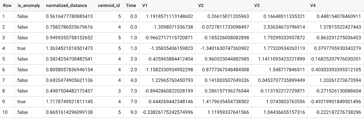
To detect anomalies in new data, use ML.DETECT_ANOMALIES and provide new data as input:
Language: SQL
SELECT*FROMML.DETECT_ANOMALIES(MODEL `mydataset.my_kmeans_model`,STRUCT(0.02 AS contamination),(SELECT * FROM `mydataset.newdata`));

How does anomaly detection work for k-means clustering models?
Anomalies are identified based on the value of each input data point’s normalized distance to its nearest cluster, which, if exceeds a threshold determined by the contamination value, is identified as an anomaly. How does this work exactly? With a k-means model and data as inputs, ML.DETECT_ANOMALIES first computes the absolute distance for each input data point to all cluster centroids in the model, then normalizes each distance by the respective cluster radius (which is defined as the standard deviation of the absolute distances of all points in this cluster to the centroid). For each data point, ML.DETECT_ANOMALIES returns the nearest centroid_id based on normalized_distance, as seen in the screenshot above. The contamination value, specified by the user, determines the threshold of whether a data point is considered an anomaly. For example, a contamination value of 0.1 means that the top 10% of descending normalized distance from the training data will be used as the cut-off threshold. If the normalized distance for a datapoint exceeds the threshold, then it is identified as an anomaly. Setting an appropriate contamination will be highly dependent on the requirements of the user or business.
For more information on anomaly detection with k-means clustering, please see the documentation here.
Anomaly detection with an autoencoder model
You can now detect anomalies using autoencoder models, by running ML.DETECT_ANOMALIES to detect anomalies in the training data or in new input data.
Begin by creating an autoencoder model:
Language: SQL
CREATE MODEL `mydataset.my_autoencoder_model`OPTIONS(model_type='autoencoder',activation_fn='relu',batch_size=8,dropout=0.2,hidden_units=[32, 16, 4, 16, 32],learn_rate=0.001,l1_reg_activation=0.0001,max_iterations=10,optimizer='adam') ASSELECT* EXCEPT(Time, Class)FROM`bigquery-public-data.ml_datasets.ulb_fraud_detection`;
To detect anomalies in the training data, use ML.DETECT_ANOMALIES with the same data used during training:
Language: SQL
SELECT*FROMML.DETECT_ANOMALIES(MODEL `mydataset.my_autoencoder_model`,STRUCT(0.02 AS contamination),TABLE `bigquery-public-data.ml_datasets.ulb_fraud_detection`);
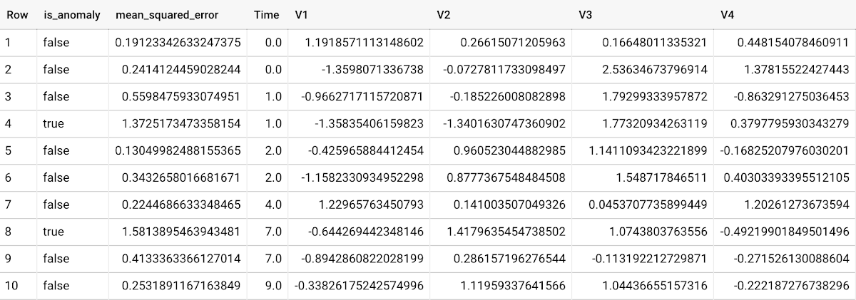
To detect anomalies in new data, use ML.DETECT_ANOMALIES and provide new data as input:
Language: SQL
SELECT*FROMML.DETECT_ANOMALIES(MODEL `mydataset.my_autoencoder_model`,STRUCT(0.02 AS contamination),(SELECT * FROM `mydataset.newdata`));

How does anomaly detection work for autoencoder models?
Anomalies are identified based on the value of each input data point’s reconstructed error, which, if exceeds a threshold determined by the contamination value, is identified as an anomaly. How does this work exactly? With an autoencoder model and data as inputs, ML.DETECT_ANOMALIES first computes the mean_squared_error for each data point between its original values and its reconstructed values. The contamination value, specified by the user, determines the threshold of whether a data point is considered an anomaly. For example, a contamination value of 0.1 means that the top 10% of descending error from the training data will be used as the cut-off threshold. Setting an appropriate contamination will be highly dependent on the requirements of the user or business.
For more information on anomaly detection with autoencoder models, please see the documentation here.
Anomaly detection with an ARIMA_PLUS time-series model
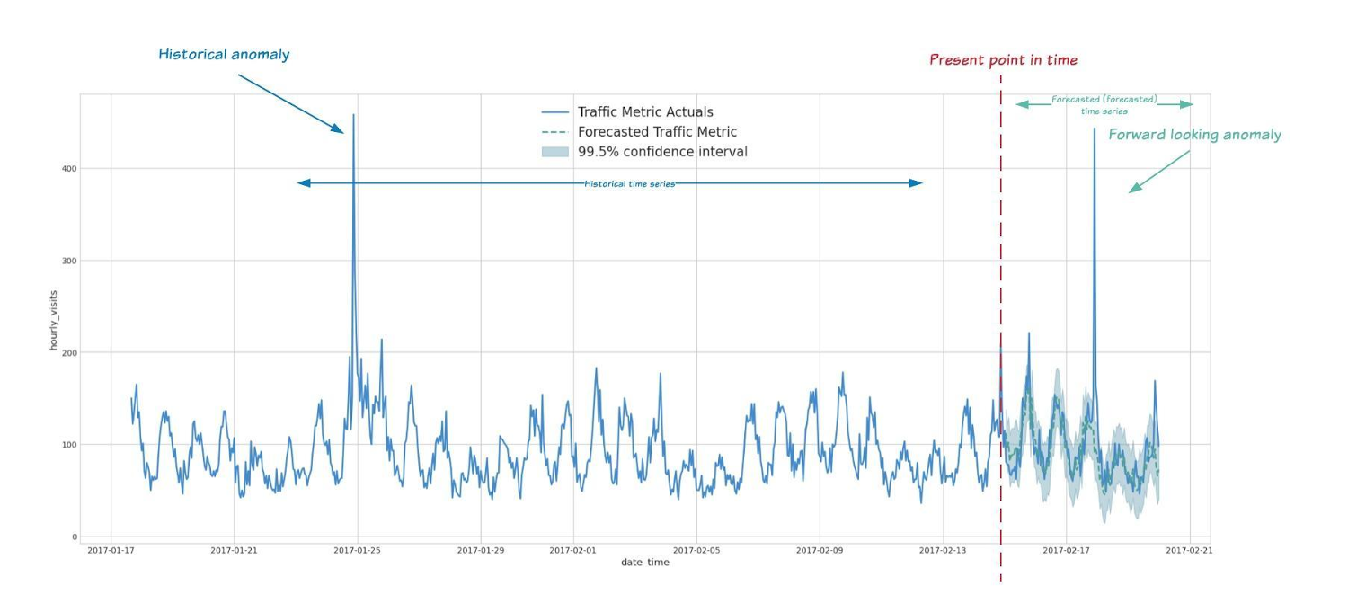
With ML.DETECT_ANOMALIES, you can now detect anomalies using ARIMA_PLUS time series models in the (historical) training data or in new input data. Here are some examples of when might you want to detect anomalies with time-series data:
Detecting anomalies in historical data:
- Cleaning up data for forecasting and modeling purposes, e.g. preprocessing historical time series before using them to train an ML model.
- When you have a large number of retail demand time series (thousands of products across hundreds of stores or zip codes), you may want to quickly identify which stores and product categories had anomalous sales patterns, and then perform a deeper analysis of why that was the case.
Forward looking anomaly detection:
- Detecting consumer behavior and pricing anomalies as early as possible: e.g. if traffic to a specific product page suddenly and unexpectedly spikes, it might be because of an error in the pricing process that leads to an unusually low price.
- When you have a large number of retail demand time series (thousands of products across hundreds of stores or zip codes), you would like to identify which stores and product categories had anomalous sales patterns based on your forecasts, so you can quickly respond to any unexpected spikes or dips.
How do you detect anomalies using ARIMA_PLUS? Begin by creating an ARIMA_PLUS time series model:
Language: SQL
CREATE OR REPLACE MODEL mydataset.my_arima_plus_modelOPTIONS(MODEL_TYPE='ARIMA_PLUS',TIME_SERIES_TIMESTAMP_COL='date',TIME_SERIES_DATA_COL='total_amount_sold',TIME_SERIES_ID_COL='item_name',HOLIDAY_REGION='US') ASSELECTdate,item_description AS item_name,SUM(bottles_sold) AS total_amount_soldFROM`bigquery-public-data.iowa_liquor_sales.sales`GROUP BYdate,item_nameHAVINGdate BETWEEN DATE('2016-01-04') AND DATE('2017-06-01')AND item_name IN ("Black Velvet", "Captain Morgan Spiced Rum","Hawkeye Vodka", "Five O'Clock Vodka", "Fireball Cinnamon Whiskey");
To detect anomalies in the training data, use ML.DETECT_ANOMALIES with the model obtained above:
Language: SQL
SELECT*FROMML.DETECT_ANOMALIES(MODEL `mydataset.my_arima_plus_model`,STRUCT(0.8 AS anomaly_prob_threshold));
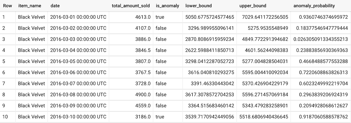
To detect anomalies in new data, use ML.DETECT_ANOMALIES and provide new data as input:
Language: SQL
WITHnew_data AS (SELECTdate,item_description AS item_name,SUM(bottles_sold) AS total_amount_soldFROM`bigquery-public-data.iowa_liquor_sales.sales`GROUP BYdate,item_nameHAVINGdate BETWEEN DATE('2017-06-02')AND DATE('2017-10-01')AND item_name IN ('Black Velvet','Captain Morgan Spiced Rum','Hawkeye Vodka',"Five O'Clock Vodka",'Fireball Cinnamon Whiskey') )SELECT*FROMML.DETECT_ANOMALIES(MODEL `mydataset.my_arima_plus_model`,STRUCT(0.8 AS anomaly_prob_threshold),(SELECT*FROMnew_data));
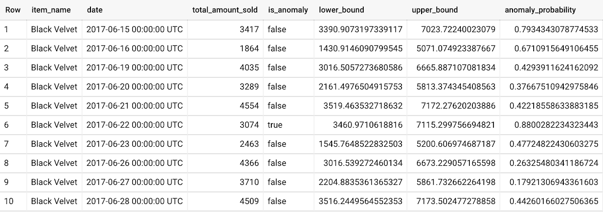
For more information on anomaly detection with ARIMA_PLUS time series models, please see the documentation here.
Thanks to the BigQuery ML team, especially Abhinav Khushraj, Abhishek Kashyap, Amir Hormati, Jerry Ye, Xi Cheng, Skander Hannachi, Steve Walker, and Stephanie Wang.
Datashare for Financial Services: Securing the Publishers and Consumers’ Access to Market Data

8572
Of your peers have already read this article.
4:30 Minutes
The most insightful time you'll spend today!
Access to the cloud has advanced the distribution and consumption of financial information on a global scale. In parallel, the global financial data landscape has been transformed by an influx of alternative data sources, including social media, meteorological data, satellite imagery, and other data. Exchanges and market data providers now find they need to include these new datasets to enrich their products and compete, which has meant they now must consider cloud-based models to keep up with the demands of their customers who expect easy, quick, flexible and cost-efficient ways to consume market data.
To address these needs, today we’re announcing the general availability of Datashare for financial services, a new Google Cloud solution that brings together the entire capital markets ecosystem—data publishers, and data consumers—to exchange market data securely and easily.
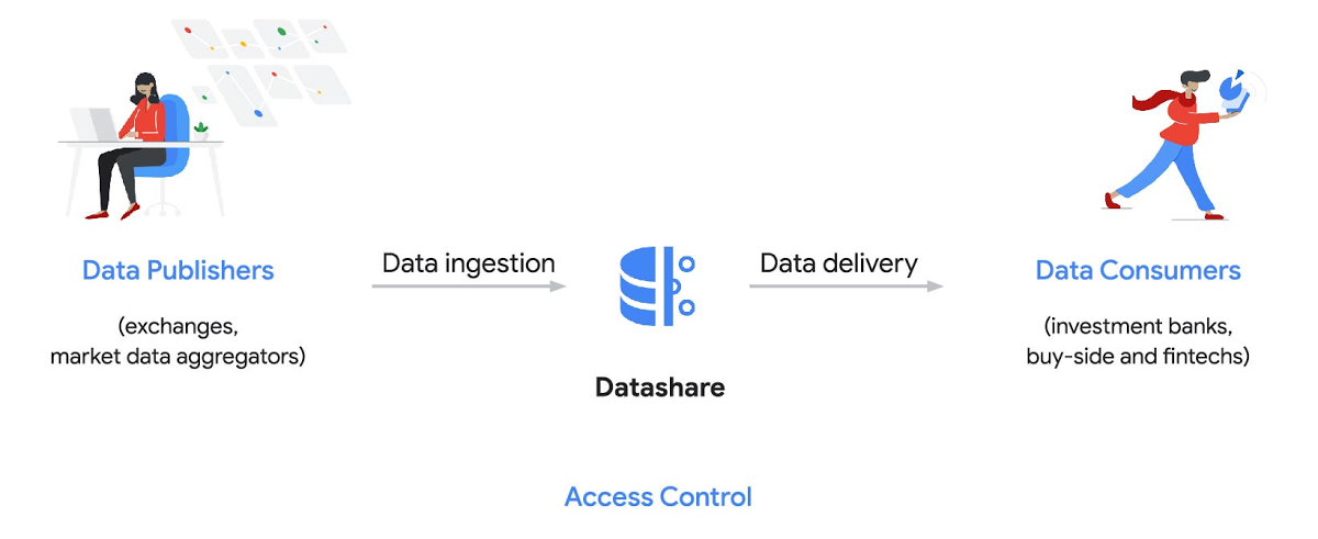
Datashare helps organize third-party financial information, making it accessible and useful to market data publishers and data consumers. We open-sourced the entire Datashare solution so market data publishers can now onboard their licensed datasets to Google Cloud securely, quickly and easily, while data consumers can consume that data as a service in tools of their preference, such as BigQuery.
Three ways to distribute and consume your data
Batch data delivery
Datashare provides a batch data delivery mechanism for data publishers to deliver their reference data, historical tick data, alternative market data sources and more via BigQuery, reducing the administrative burden on data consumers to extract insights from data.
Real-time data streaming delivery
By using this event-based data delivery channel for rapidly changing instrument prices, tick data, orders, news and others via Pub/Sub, data consumers can reliably process individual messages or rewind to a point in time to replay a prior market scenario and test model changes.
Monetizing licensed datasets
Market data publishers can onboard their licensed datasets to Google Cloud and make them available via a one-stop-shop on Google Cloud Marketplace, enabling a new sales channel to expand market reach.
Reference architecture
Check out the diagram below to see how you can share your batch and real-time data directly to your Google Cloud customers with BigQuery and Pub/Sub.

As you can see in the above reference architecture, both publishers and consumers can derive several benefits from the solution:
Benefits for data publishers
- You no longer have to maintain your own delivery and licensing infrastructure.
- You can easily package and deliver granular data products and experiments with SQL.
- You can have a solution that scales with your business as data volumes and number of customers grow.
Benefits for data consumers
- Your data is ready for analysis and machine learning (ML)— you no longer have to maintain extract, transform, and load (ETL) pipelines to load files and transform data.
- You can avoid the expense and burden of maintaining multiple copies of large data files.
- You can be more targeted with consumption of data using BigQuery queries, improving performance, and compliance, and reducing cost.
Accessing the datasets
Google Cloud has been working with multiple industry firms on innovating in the market data space. By using Datashare for publishing, data publishers can make their entire datasets available on Google Cloud. Early adopters of Datashare include firms such as OneTick and Accern. OneTick’s datasets include reference and historical futures data (that can be accessed in our console with your login). Accern’s datasets include alternative data such as market sentiment and credit analysis data (that can be accessed in our console with your login).
To make it more helpful, we partnered with Accern to create a hypothetical scenario to describe the data acquisition and analytics process step-by-step.
Accern use case
As a sustainability analyst, you require an economic, social and governance (ESG) dataset to determine which sector is the most widely covered ESG sector by analysts, and to also identify the sector with the lowest ESG sentiment score. Now, you can discover and acquire an ESG dataset in Google Cloud.
Step 1. Navigate to the Financial Services solutions page in the Google Cloud console:

Step 2. Click a dataset, for example Accern AI-Generated ESG Insights, then review the overview details, plans and pricing, documentation and support information. To view the available pricing tiers, click ‘View All Plans’. Once you’ve decided on a tier that you would like to subscribe to, click ‘Select’, choose a billing account and review and accept the terms of service to complete the subscription. Once the steps are complete, click ‘Subscribe’ at the bottom. An overlay window will appear, click ‘Register with Accern’ to activate and complete the subscription.
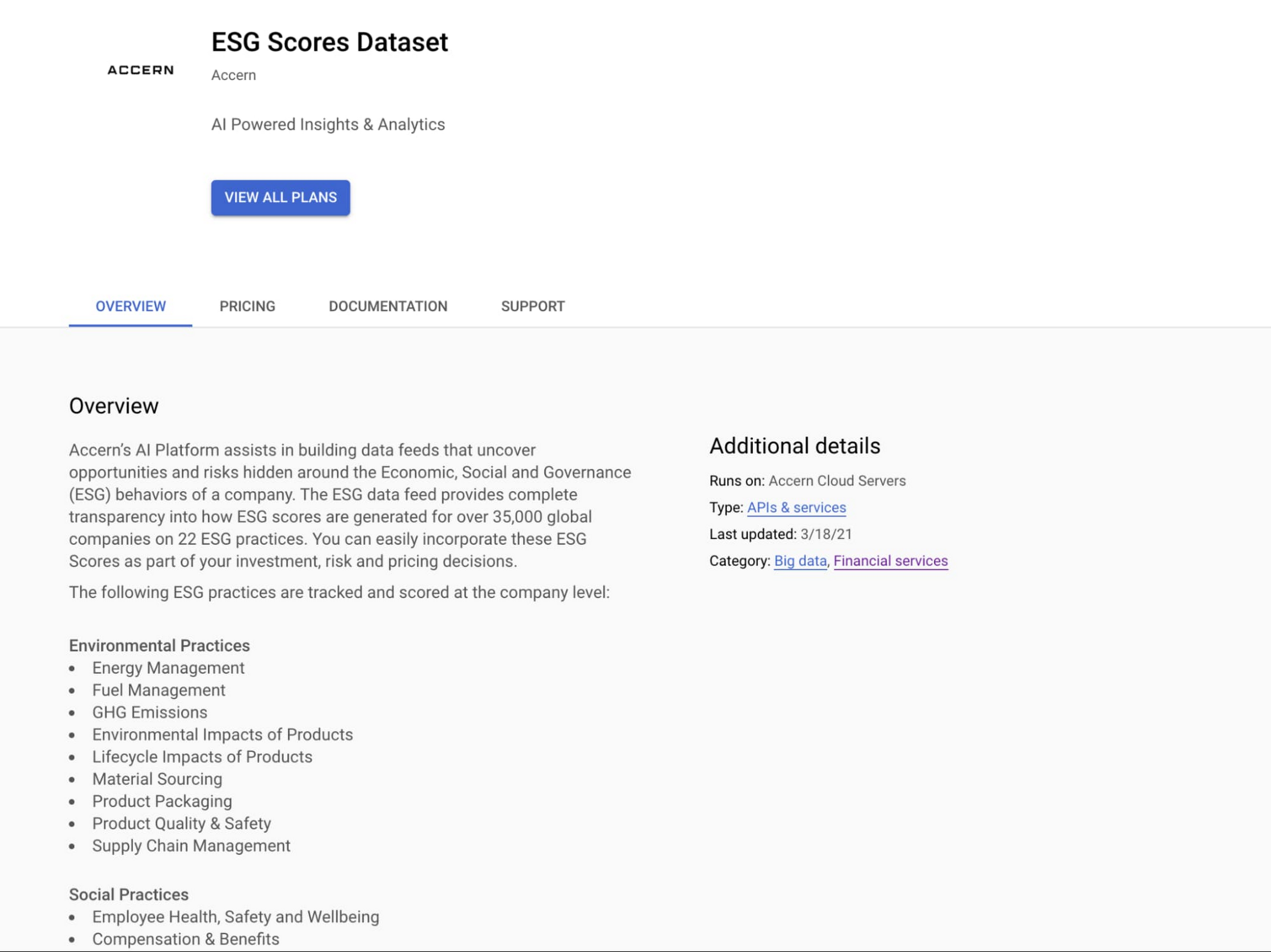

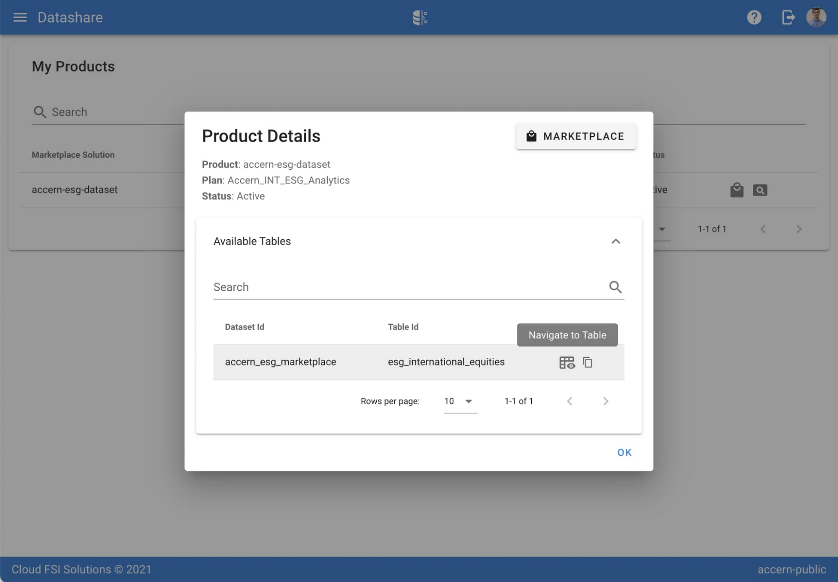
Step 3. Once activation is complete, you’ll be directed to the Datashare ‘My Products’ screen. Voila! You are now subscribed to Accern’s ESG Scores dataset and can access it in your Google Cloud instance using BigQuery. To access the data, click the hour glass icon on the corresponding ‘My Products’ record that you just purchased. An overlay will present you with the details on the dataset and/or table. Click the ‘Navigate to Table’ button to navigate through to the BigQuery console.


Step 4. Now that you have access and are in the BigQuery console, it’s time to generate data insights.
For this example, we’ve eliminated the company identifying information that is included as part of the subscription and aggregated company ESG in a view where each row represents a day, an industry sector, a specific identified ‘ESG Issues’ (event_group and event) and the respective ‘ESG Sentiment’ per issue.

For example, row 1 indicates that within the ‘Healthcare’ sector, there was a ‘Social – Civil Society’ issue identified and it had a negative ESG sentiment score of -15.35.
Step 5. Generate a report by exporting it to Data Studio to build visualizations and conduct additional analysis on the ESG data.
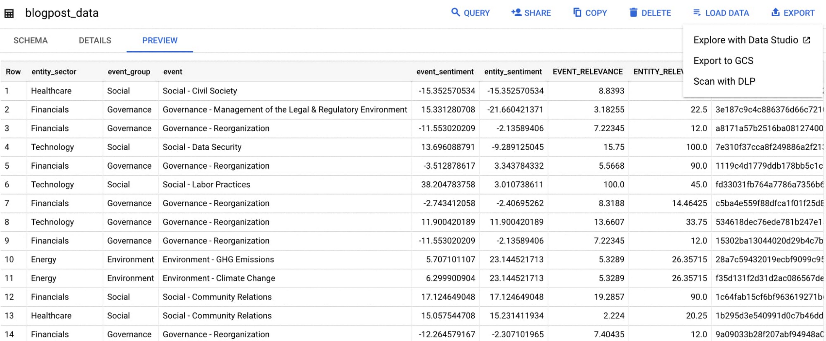
Select ‘Export’ and ‘Explore with Data Studio’.
Step 6. Build a simple/basic report.
Now that the ESG data appears in Data Studio, you can start by building a simple chart to help you understand which industry sectors have the highest volume of discussions around ESG and the overall ESG Sentiment per industry sector.
To build the chart:
- Select the chart type ‘Table’.
- Include
Entity_Sectoras your dimension to aggregate results by ‘Industry Sector.’ - Include
Signal_IDas a measure to count the number of ESG passages identified per ‘Industry Sector.’ - Include
AVG(Event_Sentiment)as a measure to display the overall ESG Sentiment per ‘Industry Sector’ across ESG Issues.

You can see sectors that are most discussed when it comes to ESG related topics and their corresponding ‘ESG Sentiment’ scores.
Step 7. Build your final report in Data Studio.
As a next step you can further drill into the data to understand ESG data specific to each ‘Industry Sector’ and identify positive and negative ESG practices.
Accern has built a more complex sample dashboard and made it available publicly here. You can interact with this report and play around with the data. The dashboard can help to identify material ESG insights for each sector to inform your investment and risk processes. If you have additional questions, you can reach out to Accern directly.

Discovering, accessing and analyzing licensed datasets is quick and easy. Stay tuned for more updates on new licensed datasets.
Publishing your data via Datashare
If you are a publisher of market data, alternative, or exotic data, you can use Datashare to get it published on Google Cloud Marketplace.
Start by joining the Partner Advantage program by registering for the Partner Advantage Portal and applying for the Partner Advantage Build Model engagement. Visit our getting started guide for information to get started on publishing licensed datasets in the Marketplace. Stay tuned for a future blog post about using Datashare to publish datasets in the Marketplace.
More solutions for capital markets
Check out other Google Cloud solutions for capital markets.
Scaling Machine Learning Operations with Vertex AI AutoML and Pipeline

2555
Of your peers have already read this article.
2:30 Minutes
The most insightful time you'll spend today!
When you build a Machine Learning (ML) product, consider at least two MLOps scenarios. First, the model is replaceable, as breakthrough algorithms are introduced in academia or industry. Second, the model itself has to evolve with the data in the changing world.
We can handle both scenarios with the services provided by Vertex AI. For example:
- AutoML capability automatically identifies the best model based on your budget, data, and settings.
- You can easily manage the dataset with Vertex Managed Datasets by creating a new dataset or adding data to an existing dataset.
- You can build an ML pipeline to automate a series of steps that start with importing a dataset and end with deploying a model using Vertex Pipelines.
This blog post shows you how to build this system. You can find the full notebook for reproduction here. Many folks focus on the ML pipeline when it comes to MLOps, but there are more parts to building MLOps as a “system”. In this post, you will see how Google Cloud Storage (GCS) and Google Cloud Functions manage data and handle events in the MLOps system.
Architecture
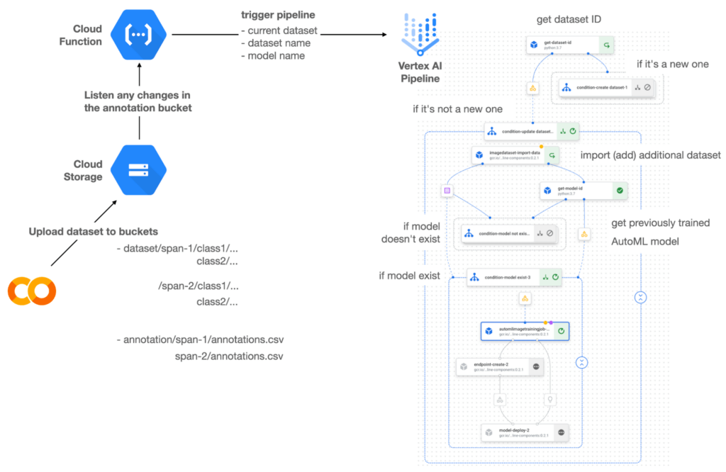

Figure 1 shows the overall architecture presented in this blog. We cover the components and their connection in the context of two common workflows of the MLOps system.
Components
Vertex AI is at the heart of this system, and it leverages Vertex Managed Datasets, AutoML, Predictions, and Pipelines. We can create and manage a dataset as it grows using Vertex Managed Datasets. Vertex AutoML selects the best model without your knowing much about modeling. Vertex Predictions creates an endpoint (RestAPI) to which the client communicates.
It is a simple, fully managed yet somewhat complete end-to-end MLOps workflow moves from a dataset to training a model that gets deployed. This workflow can be programmatically written in Vertex Pipelines. Vertex Pipelines outputs the specification for an ML pipeline allowing you to re-run the pipeline whenever or wherever you want. Specify when and how to trigger the pipeline using Cloud Functions and Cloud Storage.
Cloud Functions is a serverless way to deploy your code in Google Cloud. In this particular project, it triggers the pipeline by listening to changes on the specified Cloud Storage location. Specifically, if a new dataset is added, for example, a new span number is created; the pipeline is triggered to train the dataset, and a new model is deployed.
Workflow
This MLOps system prepares the dataset with either Vertex Dataset’s built-in user interface (UI) or any external tools based on your preference. You can upload the prepared dataset into the designated GCS bucket with a new folder named SPAN-NUMBER. Cloud Functions then detects the changes in the GCS bucket and triggers the Vertex Pipeline to run the jobs from AutoML training to endpoint deployment.
Inside the Vertex Pipeline, it checks if there is an existing dataset created previously. If the dataset is new, Vertex Pipeline creates a new Vertex Dataset by importing the dataset from the GCS location and emits the corresponding Artifact. Otherwise, it adds the additional dataset to the existing Vertex Dataset and emits an artifact.
When the Vertex Pipeline recognizes the dataset as a new one, it trains a new AutoML model and deploys it by creating a new endpoint. If the dataset isn’t new, it tries to retrieve the model ID from Vertex Model and determines whether a new AutoML model or an updated AutoML model is needed. The second branch determines whether the AutoML model has been created. If it hasn’t been created, the second branch creates a new model. Also, when the model is trained, the corresponding component emits the artifact as well.
Directory structure that reflects different distributions
In this project, I have created two subsets of the CIFAR-10 dataset, SPAN-1 and SPAN-2. A more general version of this project can be found here, which shows how to build training and batch evaluation pipelines pipelines. The pipelines can be set up to cooperate so they can evaluate the currently deployed model and trigger the retraining process.
ML Pipeline with Kubeflow Pipelines (KFP)
We chose to use Kubeflow Pipelines to orchestrate the pipeline. There are a few things that I would like to highlight. First, it’s good to know how to make branches with conditional statements in KFP. Second, you need to explore AutoML API specifications to fully leverage AutoML capabilities, such as training a model based on the previously trained one. Last, you also need to find a way to emit artifacts for Vertex Dataset and Vertex Model to consume that Vertex AI can recognize them. Let’s go through these one by one.
Branching strategy
In this project, there are two main conditions and two sub-branches inside the second main branch. The main branches split the pipeline based on a condition if there is an existing Vertex Dataset. The sub-branches are applied in the second main branch, which is selected when there is an exciting Vertex Dataset. It looks up the list of models and decides to train an AutoML model from scratch or a previously trained one.
ML pipelines written in KFP can have conditions with a special syntax of kfp.dsl.Condition. For instance, we can define the branches as follows:
from google_cloud_pipeline_components import aiplatform as gcc_aip


# try to get Vertex Dataset ID
dataset_op = get_dataset_id(...)

with kfp.dsl.Condition(name="create dataset",
                       dataset_op.outputs['Output'] == 'None'):
    # Create Vertex Dataset, train AutoML from scratch, deploy model

with kfp.dsl.Condition(name="update dataset",
                       dataset_op.outputs['Output'] != 'None'):
    # Update existing Vertex Dataset
    ...

    # try to get Vertex Model ID
    model_op = get_model_id(...)

    with kfp.dsl.Condition(name='model not exist',
                           model_op.outputs['Output'] == 'None'):
    # Create Vertex Dataset, train AutoML from scratch, deploy model

    with kfp.dsl.Condition(name='model exist',
                           model_op.outputs['Output'] != 'None'):
        # Create Vertex Dataset, train AutoML based on trained one, deploy model
get_dataset_id and get_model_id are custom KFP components used to determine if there is an existing Vertex Dataset and Vertex Model respectively. Both return “None” if a model is found and some other value if a model isn’t found. They also emit Vertex AI-aware artifacts. You will see what this means in the next section.
Emit Vertex AI-aware artifacts
Artifacts track the path of each experiment in the ML pipeline and display metadata in the Vertex Pipeline UI. When Vertex AI aware artifacts are released into in the pipeline, Vertex Pipeline UI displays links for its internal services such as Vertex Dataset, so that users can visit a web page for more information.
So how could you write a custom component to generate Vertex AI-aware artifacts? To do this, custom components should have Output[Artifact] in their parameters. Then you need to replace the resourceName of the metadata attribute with a special string format.
The following code example is the actual definition of get_dataset_id used in the previous code snippet:
@component(
    packages_to_install=["google-cloud-aiplatform",
                         "google-cloud-pipeline-components"]
)
def get_dataset_id(project_id: str,
                     location: str,
                 dataset_name: str,
                 dataset_path: str,
                      dataset: Output[Artifact]) -> str:
    from google.cloud import aiplatform
    from google.cloud.aiplatform.datasets.image_dataset import ImageDataset
    from google_cloud_pipeline_components.types.artifact_types import VertexDataset


    aiplatform.init(project=project_id, location=location)

    datasets = aiplatform.ImageDataset.list(project=project_id,
                                            location=location,
                                            filter=f'display_name={dataset_name}')

    if len(datasets) > 0:
        dataset.metadata['resourceName'] =
               f'projects/{project_id}/locations/{location}/datasets/{datasets[0].name}'
        return f'projects/{project_id}/locations/{location}/datasets/{datasets[0].name}'
    else:
        return 'None'
As you see, the dataset is defined in the parameters as Output[Artifact]. Even though it appears in the parameter, it is actually emitted automatically. You just need to provide the necessary data as if it is a function variable.
The dataset component retrieves the list of Vertex Dataset by calling the aiplotform.ImageDataset.list API. If the length of it is zero, it simply returns ‘None’. Otherwise, it returns the found resource name of the Vertex Dataset and provides the dataset.metadata[‘resourceName’] with the resource name at the same time. The Vertex AI-aware resource name follows a special string format, which is ‘projects/<project-id>/locations/<location>/<vertex-resource-type>/<resource-name>’.
The <vertex-resource-type>can be anything that points to an internal Vertex AI service. For instance, if you want to specify that the artifact is the Vertex Model, then you should replace <vertex-resource-type> with models. The <resource-name> is the unique ID of the resource, and it can be accessed in the name attribute of the resource found by the aiplatform API. The other custom component, get_model_id, is written in a very similar way as well.
AutoML based on the previous model
You sometimes want to train a new model on top of the previously best model. If that is possible, the new model will probably be much better than the one trained from scratch, because it leverages previously learned knowledge.
Luckily, Vertex AutoML comes with the ability to train a model using a previous model. AutoMLImageTrainingJobRunOp component lets you train a model by simply providing the base_model argument as follows:
training_job_run_op =
gcc_aip.AutoMLImageTrainingJobRunOp(
…,
base_model=model_op.outputs['model'],
…
)
When training a new AutoML model from scratch, you pass ‘None‘ in the base_model argument, and it is the default value. However, you can set it with a VertexModel artifact, and the component will trigger an AutoML training job based on the other model.
One thing to be careful of is that VertexModel artifacts can’t be constructed in a typical way of Python programming That means you can’t create an instance of VertexModel artifact by setting the id found in the Vertex Model dashboard. The only way you can create one is to set the metadata[‘resourceName’] parameters properly. The same rule applies to other Vertex AI-related artifacts such as VertexDataset. You can see how the VertexDataset artifact is constructed properly to get an existing Vertex Dataset to import additional data into it. See the full notebook of this project here.
Cost
You can reproduce the same result from this project with the free $300 credit when you create a new GCP account.
At the time of this blog post, Vertex Pipelines costs about $0.03/run, and the type of underlying VM for each pipeline component is e2-standard-4, which costs about $0.134/hour. Vertex AutoML training costs about $3.465/hour for image classification. GCS holds the actual data, which costs about $2.40/month for 100GiB capacity, and Vertex Dataset is free.
To simulate two different branches, the entire experiment took about one to two hours, and the total cost for this project is approximately $16.59. Please find more detailed pricing information about Vertex AI here.
Conclusion
Many people underestimate the capability of AutoML, but it is a great alternative for app and service developers who have little ML background. Vertex AI is a great platform that provides AutoML as well as Pipeline features to automate the ML workflow. In this article, I have demonstrated how to set up and run a basic MLOps workflow, from data injection to training a model based on the previously-achieved best one, to deploying the model to a Vertex AI platform. With this, we can let our ML model automatically adapt to the changes in a new dataset. What’s left for you to implement is to integrate a model monitoring system to detect data/model drift. One example is found here.
Cohere uses Google Cloud’s new TPU v4 Pods on its quest to create larger and more powerful language models

2817
Of your peers have already read this article.
3:30 Minutes
The most insightful time you'll spend today!
Over the past few years, advances in training large language models (LLMs) have moved natural language processing (NLP) from a bleeding-edge technology that few companies could access, to a powerful component of many common applications. From chatbots to content moderation to categorization, a general rule for NLP is that the larger the model, the greater the accuracy it’s able to achieve in understanding and generating language.
But in the quest to create larger and more powerful language models, scale has become a major challenge. Once a model becomes too large to fit on a single device, it requires distributed training strategies, which in turn require extensive compute resources with vast memory capacity and fast interconnects. You also need specialized algorithms to optimize the hardware and time resources.
Cohere engineers are working on solutions to this scaling challenge that have already yielded results. Cohere provides developers a platform for working with powerful LLMs without the infrastructure or deep ML expertise that such projects typically require. In a new technical paper, Scalable Training of Language Models using JAX pjit and TPUv4, engineers at Cohere demonstrate how their new FAX framework deployed on Google Cloud’s recently announced Cloud TPU v4 Pods addresses the challenges of scaling LLMs to hundreds of billions of parameters. Specifically, the report reveals breakthroughs in training efficiency that Cohere was able to achieve through tensor and data parallelism.
This framework aims to accelerate the research, development, and production of large language models with two significant improvements: scalability and rapid prototyping. Cohere will be able to improve its models by training larger ones more quickly, delivering better models to its customers faster. The framework also supports rapid prototyping of models that address specific objectives — for example, creating a generative model that powers customer-service chatbot — by experimenting and testing new ideas. The ability to switch back and forth among model types and optimize for different objectives will ultimately allow Cohere to offer models optimized for particular use cases.
The FAX framework relies heavily on the partitioned just-in-time compilation (pjit) feature of JAX, which abstracts the relationship between device and workload. This allows Cohere engineers to optimize efficiency, and performance by aligning devices and processes in the ideal configuration for the task at hand. Pjit works by compiling an arbitrary function into a single program (an XLA computation), that runs on multiple devices — even those residing on different hosts.
Cohere’s new solution also takes advantage of Google Cloud’s new TPU v4 Pods to perform tensor parallelism. which is more efficient than the earlier pipeline parallelism implementation. As the name suggests, the pipeline parallel approach uses accelerators in a linear fashion to scale a workload, like a single long assembly line. Accelerators must process each micro-batch of data before passing it along to the next one, and then run the backward pass in reverse order.
Tensor parallelism eliminates the accelerator idle time of pipeline parallelism, also known as the pipeline bubble. Tensor parallelism involves partitioning large tensors (mathematical arrays that define the relationship among multiple objects such as the words in a paragraph) across accelerators to perform computations at the same time on multiple devices. If pipeline parallelism is an ever-lengthening assembly line, tensor parallelism is a series of parallel assembly lines — one making the engine, the other the body, etc. — that simultaneously come together to form a complete car in a fraction of the time.
These computations are then collated, a process made practical thanks to Google Cloud TPU v4 VMs, which more than double the computational power. The superior performance of v4 chips has enabled Cohere to iterate on ideas and validate them 1.7X faster in computation than before.
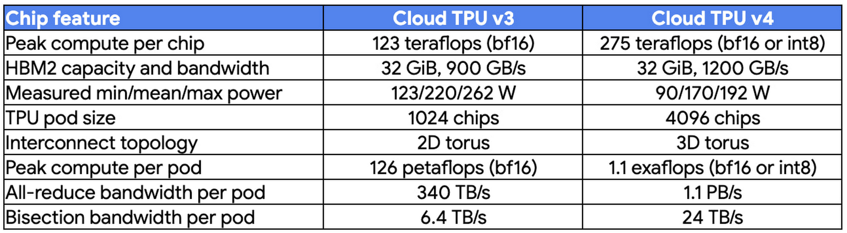
At Cohere, we build cutting-edge natural language processing (NLP) services, including APIs for language generation, classification, and search. These tools are built on top of a set of language models that Cohere trains from scratch on Cloud TPUs using JAX. We saw a 70% improvement in training time for our largest model when moving from Cloud TPU v3 Pods to Cloud TPU v4 Pods, allowing faster iterations for our researchers and higher quality results for our customers. The exceptionally low carbon footprint of Cloud TPU v4 Pods was another key factor for us.
Aidan Gomez
CEO and co-founder, Cohere
Why Google Cloud for LLM training?
As part of a multiyear technology partnership, Cohere leverages Google Cloud’s advanced AI and ML infrastructure to power its platform. Cohere develops and deploys its products on Cloud TPUs, Google Cloud’s custom-designed machine learning chips that are optimized for large-scale ML. Cohere’s recently announced their new model improvements and scalability by training an LLM using FAX on Google Cloud TPUs, and this model has demonstrated that transitioning from TPU v3 to TPU v4 has so far enabled them to achieve a total speedup of 1.7x. In addition to a significant performance boost, TPUs provide an excellent user experience with the new TPU VM architecture. Importantly, Google Cloud ensures that Cohere’s state-of-the-art ML training is achieved with the highest standards of sustainability, powered by 90% carbon-free energy in the world’s largest publicly available ML hub.
By adopting Cloud TPUs, Cohere is making LLM training faster, more economical, and more agile. This helps them provide larger and more accurate LLMs to developers, and put NLP technology in the hands of developers and businesses of all sizes.
To learn more about these LLM training advances, you can read the full paper, Scalable Training of Language Models using JAX pjit and TPUv4. To learn more about Cohere’s best practices and AI principles, you can check this article co-authored with Open AI and AI 21 Labs.
Analytics Hub for Secure Data Sharing and Analytics Unlocks True Data Value and Insights

6750
Of your peers have already read this article.
2:30 Minutes
The most insightful time you'll spend today!
Customers tell us that sharing and exchanging data with other organizations is a critical element of their analytics strategy, but it’s hamstrung by unreliable data and processes, and only getting harder with security threats and privacy regulations on the rise.
Furthermore, traditional data sharing techniques use batch data pipelines that are expensive to run, create late arriving data, and can break with any changes to the source data. They also create multiple copies of data, which brings unnecessary costs and can bypass data governance processes. These techniques do not offer features for data monetization, such as managing subscriptions and entitlements. Altogether, these challenges mean that organizations are unable to realize the full potential of transforming their business with shared data.
To address these limitations, we are introducing Analytics Hub, a new fully managed service, available in Q3, in preview, that helps you unlock the value of data sharing, leading to new insights and increased business value. With Analytics Hub you get:
- A rich data ecosystem by publishing and subscribing to analytics-ready datasets.
- Control and monitoring over how your data is being used, because data is shared in one place.
- A self-service way to access valuable and trusted data assets, including data provided by Google. For example, a unique dataset from Google Search Trends will be available, that you can query and combine with your own data.
- An easy way to monetize your data assets without the overhead of building and managing the infrastructure.
Built on a decade of cross-organizational sharing
While Analytics Hub is a new service, it builds on BigQuery, Google’s petabyte-scale, serverless cloud data warehouse. BigQuery’s unique architecture provides separation between compute and storage, enabling data publishers to share data with as many subscribers as you want without having to make multiple copies of your data. With BigQuery, there are no servers to deploy or manage, which means that data consumers get immediate value from shared data. Data can be provided and consumed in real-time using the streaming capabilities of BigQuery and you can leverage the built in machine learning, geospatial, and natural language capabilities of BigQuery or take advantage of the native business intelligence support with tools like Looker, Google Sheets, and Data Studio.
BigQuery has had cross-organizational, in-place data sharing capabilities since it was introduced in 2010. We took a look at usage metrics in BigQuery and found that over a 7 day period in April, we had over 3,000 different organizations sharing over 200 petabytes of data. These numbers don’t include data sharing between departments within the same organization.
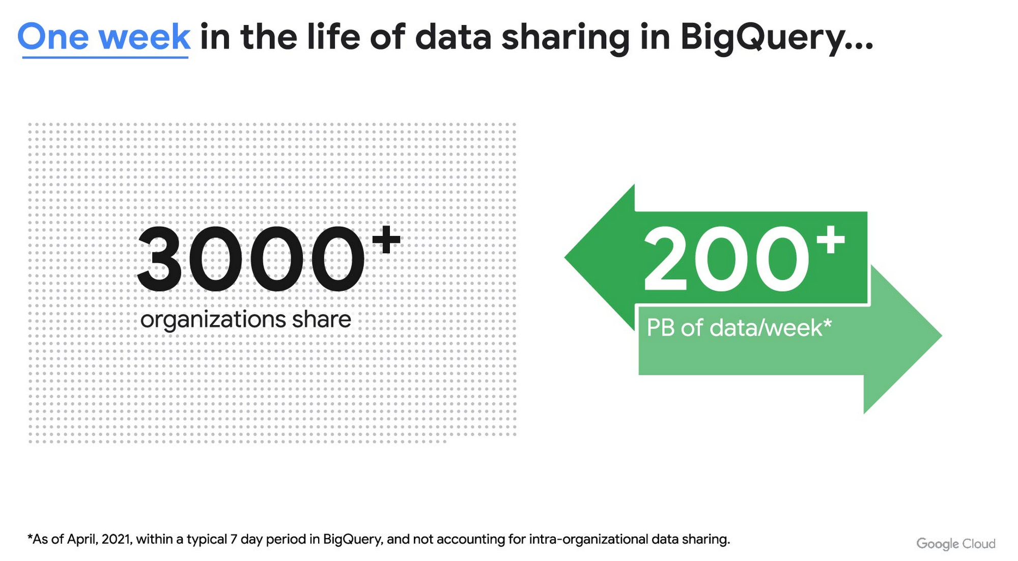
As you can see, data sharing in BigQuery is already popular. But we want to make it easier and even more scalable.
Raising the bar on data sharing
To make data sharing easier and more scalable in BigQuery, Analytics Hub introduces the concepts of shared datasets and exchanges. As a data publisher, you create shared datasets that contain the views of data that you want to deliver to your subscribers. Next, you create exchanges, which are used to organize and secure shared datasets. By default, exchanges are completely private, which means that only the users and groups that you give access to can view or subscribe to the data. You can also create internal exchanges or leverage public exchanges provided by Google. Finally, you publish shared datasets into an exchange to make them available to subscribers.
Data subscribers search through the datasets that are available across all exchanges for which they have access and subscribe to relevant datasets. This creates a linked dataset in their project that they can query and join with their own data. Subscribers pay for the queries that they run against the data while the publisher pays for the storage of the data. Data providers can add new data, new tables, or new columns to the shared dataset and these will be immediately available to subscribers. In addition, the publisher can track subscribers, disable subscriptions, and see aggregated usage information for the shared data.
Analytics Hub makes it easy for you to publish, discover, and subscribe to valuable datasets that you can combine with your own data to derive unique insights. Here are some types of data that will be available through Analytics Hub:
- Public datasets: Easy access to the existing repository of over 200 public datasets, including data about weather and climate, cryptocurrency, healthcare and life sciences, and transportation.
- Google datasets: Unique, freely-available datasets from Google. One example of this is the COVID-19 community mobility dataset. Another example is the forthcoming Google Trends dataset, which will provide the top 25 search terms and top 25 rising search terms over a 5 year window in 210 distinct locations in the US. Trends data can be used by everyone in the organization to gain insights into what customers care about.
- Commercial (paid for) datasets: We are working with leading commercial data providers to bring their data products to Analytics Hub. If you are interested in delivering your data via Analytics Hub, we’re also introducing Data Gravity, an initiative that provides storage benefits and new distribution paths for data published through Analytics Hub.
- Internal datasets: We know that data sharing can be challenging in larger organizations. Analytics Hub can be used for internal data, for example, to share standardized customer demographics with your sales engineering and data science teams.
Customers and partners using Analytics Hub

“Google Search Trends data has always been an important tool for our WPP agency data teams. At WPP we believe that data variety is a superpower which is why we are excited to use the new Trends dataset availability within BigQuery, plus the launch of Analytics Hub. The best creativity in the world is informed by data insights, and influenced by what people search for, so the operational efficiencies we’ll gain via the Analytics Hub and the insights we can drive with Trends data are just phenomenal.”
—Di Mayze Global Head of Data and AI, WPP

“Equifax Ignite is our shared data analytics environment within our Equifax data fabric. We are excited to partner with Google to leverage Analytics Hub and BigQuery to deliver data to over 400 statisticians and data modelers as well as securely sharing data with our partner financial institutions.”
—Kumar Menon, SVP Data Fabric and Decision Science, Equifax

“The flow of data and insights between our teams at Deloitte and our clients is paramount for building truly transformational data cultures. With its purpose-built architecture for secure data exchanges and sharing analytics resources, Google Cloud’s Analytics Hub can help provide significant operational efficiencies for how Deloitte teams support our clients’ data-driven initiatives within their industry ecosystems. It will also help minimize the worries about scale, privacy and security, or the administrative burden associated with each.”
—Navin Warerkar, Managing Director, Deloitte Consulting LLP, and US Google Cloud Data & Analytics GTM Lead

“Crux Informatics is proud to partner with Google to support the launch of Analytics Hub, removing friction for those who need access to analytics-ready data. With thousands of datasets from over 140 sources, Crux Informatics will accelerate access to data on Analytics Hub and together provide a more efficient and cost effective solution to deliver datasets in Google Cloud’s ecosystem.”
—Will Freiberg, CEO, Crux Informatics
Next steps for Analytics Hub
This is just the beginning for Analytics Hub. As we get to preview and general availability, we will be adding additional capabilities, including workflows for publishing and subscribing, publishing analytics assets (Looker Blocks, Data Studio reports, Connected Google Sheets) along with the shared data, the ability for data publishers to specify query restrictions on the usage of their data, and making it easy for data publishers to create sandbox environments for subscribers to work with their data, even if they are not yet on Google Cloud. We will provide features in Analytics Hub for monetization of data, including managing subscriptions, data entitlements, and billing.
Please sign up for the preview, which is scheduled to be available in the third quarter of 2021. In the meantime, you can learn more about BigQuery and how to leverage its built-in data sharing capabilities. Please go to g.co/cloud/analytics-hub to register your interest in Analytics Hub.
More Relevant Stories for Your Company

Gyfted: Finding the Right Man for the Job Using Google Cloud AI/ML Tools
It’s no secret that many organizations and job seekers find the hiring process exhausting. It can be time consuming, costly, and somewhat risky for both parties. Those are just some of the experiences we wanted to change when we started Gyfted, a pre-vetted talent marketplace for people who complete tech

Candidate360: Google Cloud and Deloitte Product Improves Universities’ Enrollment and Admission Processes
Given the May 1 deadline for students to enroll, colleges and universities have been carefully watching the numbers of students who put down deposits and commit to a school. Like nearly every other sector in the U.S., colleges and universities have been hit hard by the pandemic and economic downturn,


Contact Center AI: The State of the Union
Did you know 31% of CIOs say that they have already deployed conversational AI platforms? And that this represents a 50% year on year growth? Much of this is driven by customer preferences. By 2023, customers will prefer speech interfaces to initiate self-service activities. Additionally, by 2023, 40 percent of

BigQuery Explainable AI for Demystifying the Inner Workings of ML Models. Now GA!
Explainable AI (XAI) helps you understand and interpret how your machine learning models make decisions. We're excited to announce that BigQuery Explainable AI is now generally available (GA). BigQuery is the data warehouse that supports explainable AI in a most comprehensive way w.r.t both XAI methodology and model types. It does this at
