





BigQuery Explainable AI for Demystifying the Inner Workings of ML Models. Now GA!

6565
Of your peers have already read this article.
2:00 Minutes
The most insightful time you'll spend today!
Explainable AI (XAI) helps you understand and interpret how your machine learning models make decisions. We’re excited to announce that BigQuery Explainable AI is now generally available (GA). BigQuery is the data warehouse that supports explainable AI in a most comprehensive way w.r.t both XAI methodology and model types. It does this at BigQuery scale, enabling millions of explanations within seconds with a single SQL query.
Why is Explainable AI so important? To demystify the inner workings of machine learning models, Explainable AI is quickly becoming an essential and growing need for businesses as they continue to invest in AI and ML. With 76% of enterprises now prioritizing artificial intelligence (AI) and machine learning (ML) over other initiatives in 2021 IT budgets, the majority of CEOs (82%) believe that AI-based decisions must be explainable to be trusted according to a PwC survey.
While the focus of this blogpost is on BigQuery Explainable AI, Google Cloud provides a variety of tools and frameworks to help you interpret models outside of BigQuery, such as with Vertex Explainable AI, which includes AutoML Tables, AutoML Vision, and custom-trained models.
So how does Explainable AI in BigQuery work exactly? And how might you use it in practice?
Two types of Explainable AI: global and local explainability
When it comes to Explainable AI, the first thing to note is that there are two main types of explainability as they relate to the features used to train the ML model: global explainability and local explainability.
Imagine that you have a ML model that predicts housing price (as a dollar amount), based on three features: (1) number of bedrooms, (2) distance to the nearest city center, and (3) construction date.
Global explainability (a.k.a. global feature importance) describes the features’ overall influence on the model and helps you understand if a feature had a greater influence than other features over the model’s predictions. For example, global explainability can reveal that the number of bedrooms and distance to city center typically has a much stronger influence than the construction date on predicting housing prices. Global explainability is especially useful if you have hundreds or thousands of features and you want to determine which features are the most important contributors to your model. You may also consider using global explainability as a way to identify and prune less important features to improve the generalizability of their models.
Local explainability (a.k.a. feature attributions) describes the breakdown of how each feature contributes towards a specific prediction. For example, if the model predicts that house ID#1001 has a predicted price of $230,000, local explainability would describe a baseline amount (e.g. $50,000) and how each of the features contributes on top of the baseline towards the predicted price. For example, the model may say that on top of the baseline of $50,000, having 3 bedrooms contributed an additional $50,000, close proximity to the city center added $100,000, and construction date of 2010 added $30,000, for a total predicted price of $230,000. In essence, understanding the exact contribution of each feature used by the model to make each prediction is the main purpose of local explainability.
What ML models does BigQuery Explainable AI apply to?
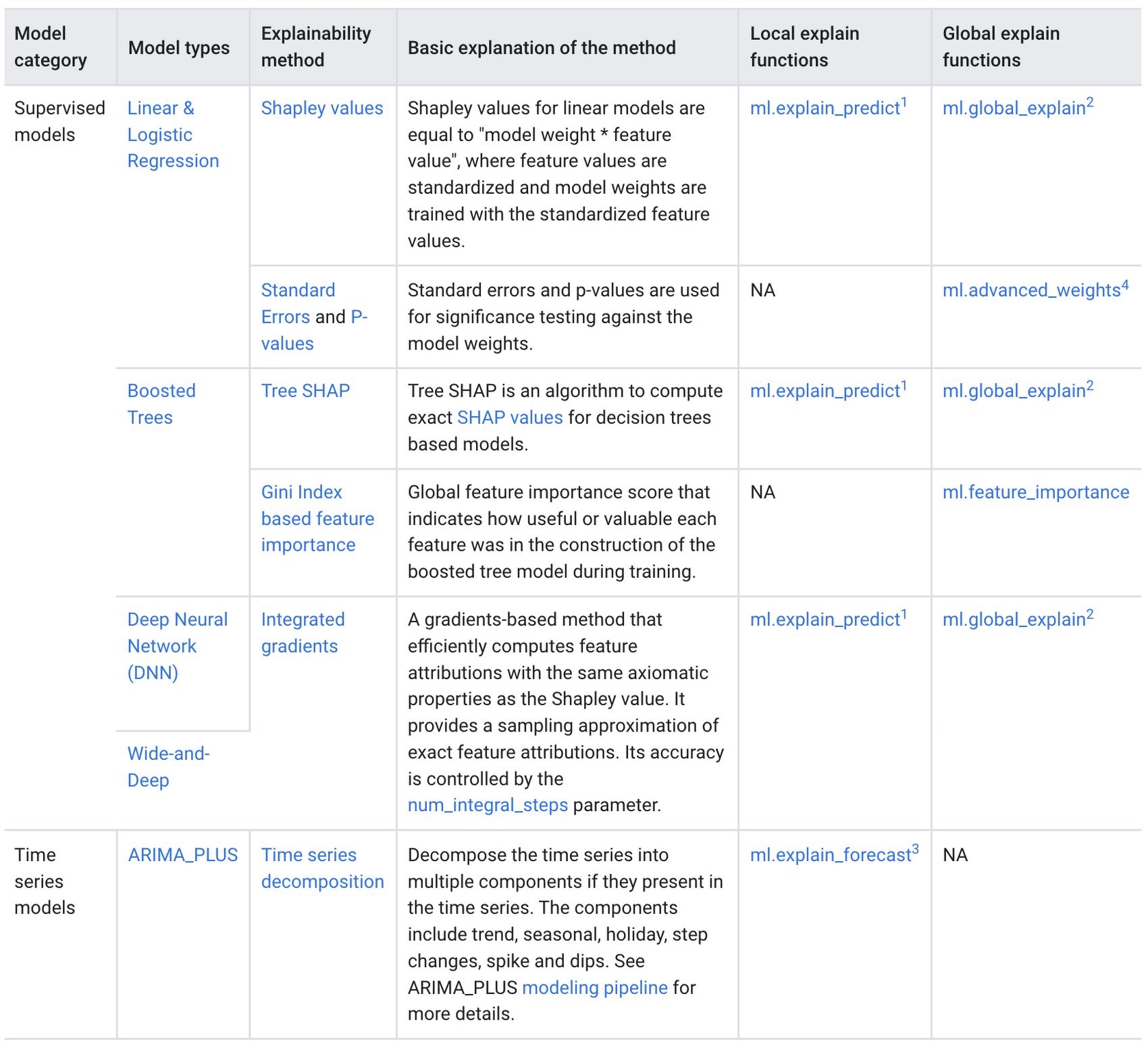
BigQuery Explainable AI applies to a variety of models, including supervised learning models for IID data and time series models. The documentation for BigQuery Explainable AI provides an overview of the different ways of applying explainability per model. Note that each explainability method has its own way of calculation (e.g. Shapley values), which are covered more in-depth in the documentation.
Examples with BigQuery Explainable AI
In this next section, we will show three examples of how to use BigQuery Explainable AI in different ML applications:
Regression models with BigQuery Explainable AI
Let’s use a boosted tree regression model to predict how much a taxi cab driver will receive in tips for a taxi ride, based on features such as number of passengers, payment type, total payment and trip distance. Then let’s use BigQuery Explainable AI to help us understand how the model made the predictions in terms of global explainability (which features were most important?) and local explainability (how did the model arrive at each prediction?).
The taxi trips dataset comes from the BigQuery public datasets and is publicly available in the table: bigquery-public-data.new_york_taxi_trips.tlc_yellow_trips_2018.
First, you can train a boosted tree regression model.
CREATE OR REPLACE MODEL bqml_tutorial.taxi_tip_regression_modelOPTIONS (model_type='boosted_tree_regressor',input_label_cols=['tip_amount'],max_iterations = 50,tree_method = 'HIST',subsample = 0.85,enable_global_explain = TRUE) ASSELECTvendor_id,passenger_count,trip_distance,rate_code,payment_type,total_amount,tip_amountFROM`bigquery-public-data.new_york_taxi_trips.tlc_yellow_trips_2018`WHERE tip_amount >= 0LIMIT 1000000
Now let’s do a prediction using ML.PREDICT, which is the standard way in BigQuery ML to make predictions without explainability.
SELECT *FROMML.PREDICT(MODEL bqml_tutorial.taxi_tip_regression_model,(SELECT"0" AS vendor_id,1 AS passenger_count,CAST(5.85 AS NUMERIC) AS trip_distance,"0" AS rate_code,"0" AS payment_type,CAST(55.56 AS NUMERIC) AS total_amount))

But you might wonder—how did the model generate this prediction of ~11.077?
BigQuery Explainable AI can help us answer this question. Instead of using ML.PREDICT, you use ML.EXPLAIN_PREDICT with an additional optional parameter top_k_features. ML.EXPLAIN_PREDICT extends the capabilities of ML.PREDICT by outputting several additional columns that explain how each feature contributes to the predicted value. In fact, since ML.EXPLAIN_PREDICT includes all the output from ML.PREDICT anyway, you may want to consider using ML.EXPLAIN_PREDICT every time instead.
SELECT *FROMML.EXPLAIN_PREDICT(MODEL bqml_tutorial.taxi_tip_regression_model,(SELECT"0" AS vendor_id,1 AS passenger_count,CAST(5.85 AS NUMERIC) AS trip_distance,"0" AS rate_code,"0" AS payment_type,CAST(55.56 AS NUMERIC) AS total_amount),STRUCT(6 AS top_k_features))
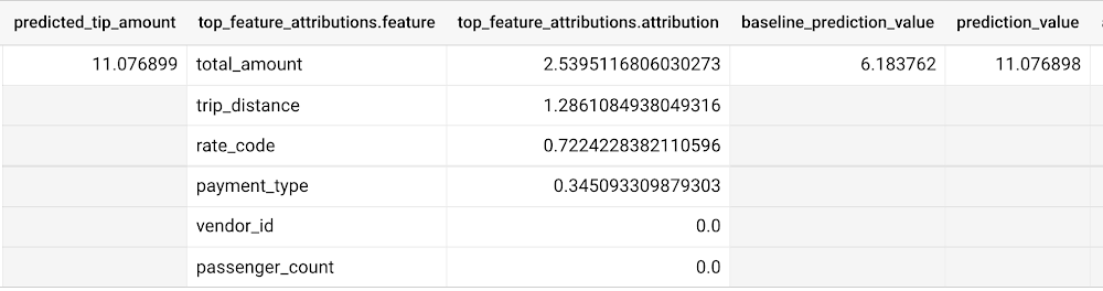
The way to interpret these columns is:
Σfeature_attributions + baseline_prediction_value = prediction_value
Let’s break this down. The prediction_value is ~11.077, which is simply the predicted_tip_amount. The baseline_prediction_value is ~6.184, which is the tip amount for an average instance. top_feature_attributions indicates how much each of the features contributes towards the prediction value. For example, total_amount contributes ~2.540 to the predicted_tip_amount.
ML.EXPLAIN_PREDICT provides local feature explainability for regression models. For global feature importance, see the documentation for ML.GLOBAL_EXPLAIN.
Classification models with BigQuery Explainable AI
Let’s use a logistic regression model to show you an example of BigQuery Explainable AI with classification models. We can use the same public dataset as before: bigquery-public-data.new_york_taxi_trips.tlc_yellow_trips_2018.
Train a logistic regression model to predict the bracket of the percentage of the tip amount out of the taxi bill.
CREATE OR REPLACE MODEL bqml_tutorial.taxi_tip_classification_modelOPTIONS(model_type='logistic_reg',input_label_cols=['tip_bucket'],enable_global_explain=true) ASSELECTvendor_id,passenger_count,trip_distance,rate_code,payment_type,total_amount,CASEWHEN tip_amount > total_amount*0.20 THEN '20% or more'WHEN tip_amount > total_amount*0.15 THEN '15% to 20%'WHEN tip_amount > total_amount*0.10 THEN '10% to 15%'ELSE '10% or less'END AS tip_bucketFROM`bigquery-public-data.new_york_taxi_trips.tlc_yellow_trips_2018`WHERE tip_amount >= 0LIMIT 1000000
Next, you can run ML.EXPLAIN_PREDICT to get both the classification results and the additional information for local feature explainability. For global explainability, you can use ML.GLOBAL_EXPLAIN. Again, since ML.EXPLAIN_PREDICT includes all the output from ML.PREDICT anyway, you may want to consider using ML.EXPLAIN_PREDICT every time instead.
SELECT *FROMML.EXPLAIN_PREDICT(MODEL bqml_tutorial.taxi_tip_classification_model,(SELECT"0" AS vendor_id,1 AS passenger_count,CAST(5.85 AS NUMERIC) AS trip_distance,"0" AS rate_code,"0" AS payment_type,CAST(55.56 AS NUMERIC) AS total_amount),STRUCT(6 AS top_k_features))
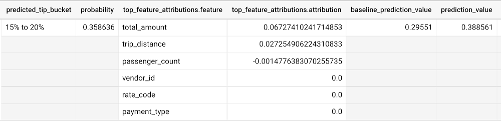
Similar to the regression example earlier, the formula is used to derive the prediction_value:
Σfeature_attributions + baseline_prediction_value = prediction_value
As you can see in the screenshot above, the baseline_prediction_value is ~0.296. total_amount is the most important feature in making this specific prediction, contributing ~0.067 to the prediction_value, though followed by trip_distance. The feature passenger_count contributes negatively to prediction_value by -0.0015. The features vendor_id, rate_code, and payment_type did not seem to contribute much to the prediction_value.
You may wonder why the prediction_value of ~0.389 doesn’t equal the probability value of ~0.359. The reason is that unlike for regression models, for classification models, prediction_value is not a probability score. Instead, prediction_value is the logit value (i.e., log-odds) for the predicted class, which you could separately convert to probabilities by applying the softmax transformation to the logit values. For example, a three-class classification has a log-odds output of [2.446, -2.021, -2.190]. After applying the softmax transformation, the probability of these class predictions is [0.9905, 0.0056, 0.0038].
Time-series forecasting models with BigQuery Explainable AI
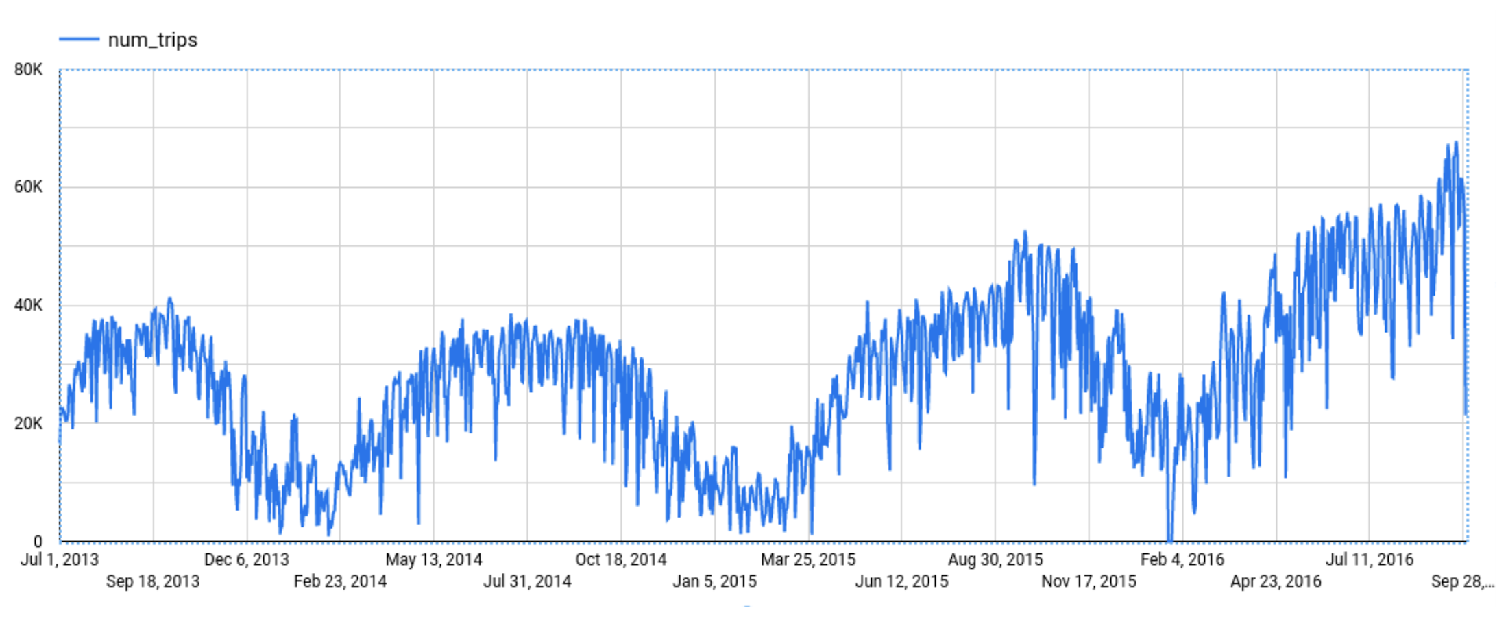
Explainable AI for forecasting provides more interpretability into how the forecasting model came to its predictions. Let’s go through an example of forecasting the number of bike trips in NYC using the new_york.citibike_trips public data in BigQuery.
You can train a time-series model ARIMA_PLUS:
CREATE OR REPLACE MODEL bqml_tutorial.nyc_citibike_arima_modelOPTIONS(model_type = 'ARIMA_PLUS',time_series_timestamp_col = 'date',time_series_data_col = 'num_trips',holiday_region = 'US') ASSELECTEXTRACT(DATE from starttime) AS date,COUNT(*) AS num_tripsFROM`bigquery-public-data.new_york.citibike_trips`GROUP BY dateNext, you can first try forecasting without explainability using ML.FORECAST:SELECT*FROMML.FORECAST(MODEL bqml_tutorial.nyc_citibike_arima_model,STRUCT(365 AS horizon, 0.9 AS confidence_level))
This function outputs the forecasted values and the prediction interval. Plotting it in addition to the input time series gives the following figure.
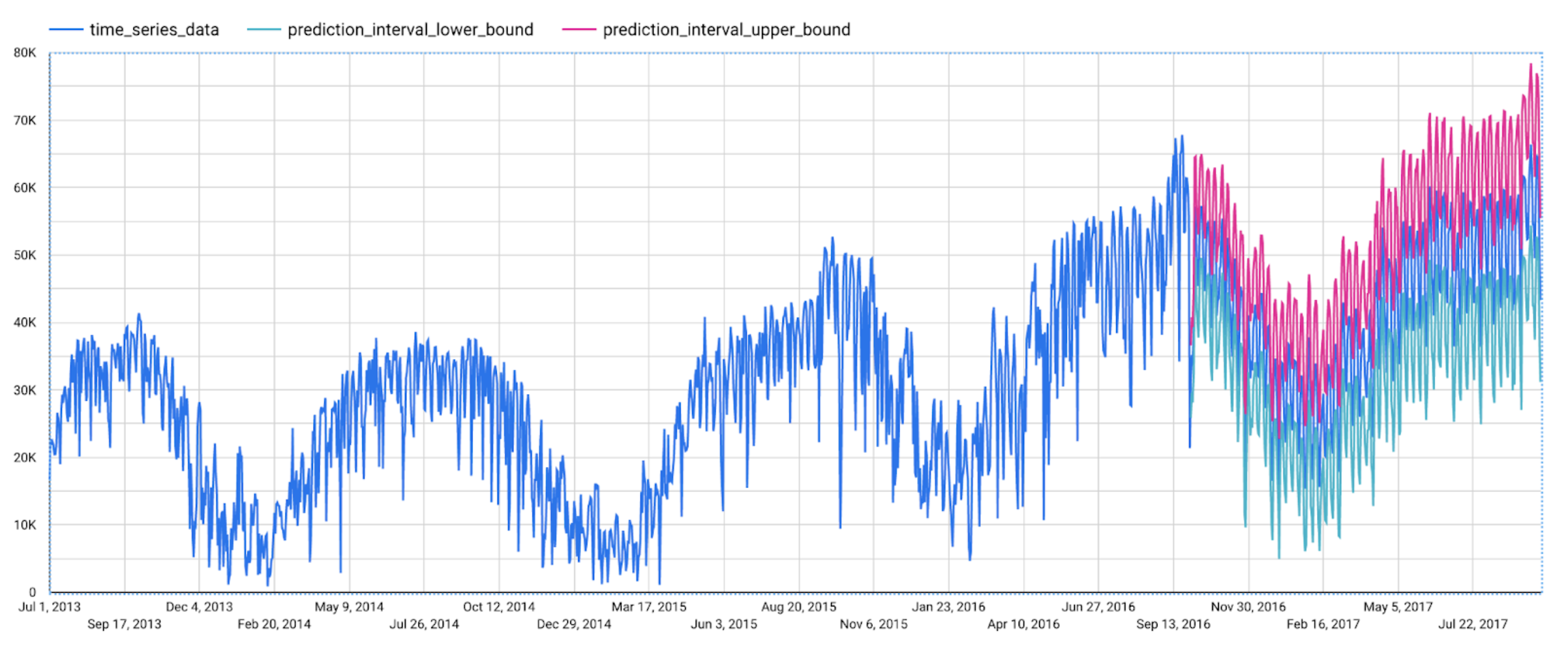
But how does the forecasting model arrive at its predictions? Explainability is especially important if the model ever generates unexpected results.
With ML.EXPLAIN_FORECAST, BigQuery Explainable AI provides extra transparency into the seasonality, trend, holiday effects, level (step) changes, and spikes and dips outlier removal. In fact, since ML.EXPLAIN_FORECAST includes all the output from ML.FORECAST anyway, you may want to consider using ML.EXPLAIN_FORECAST every time instead.
SELECT*FROMML.EXPLAIN_FORECAST(MODEL bqml_tutorial.nyc_citibike_arima_model,STRUCT(365 AS horizon, 0.9 AS confidence_level))
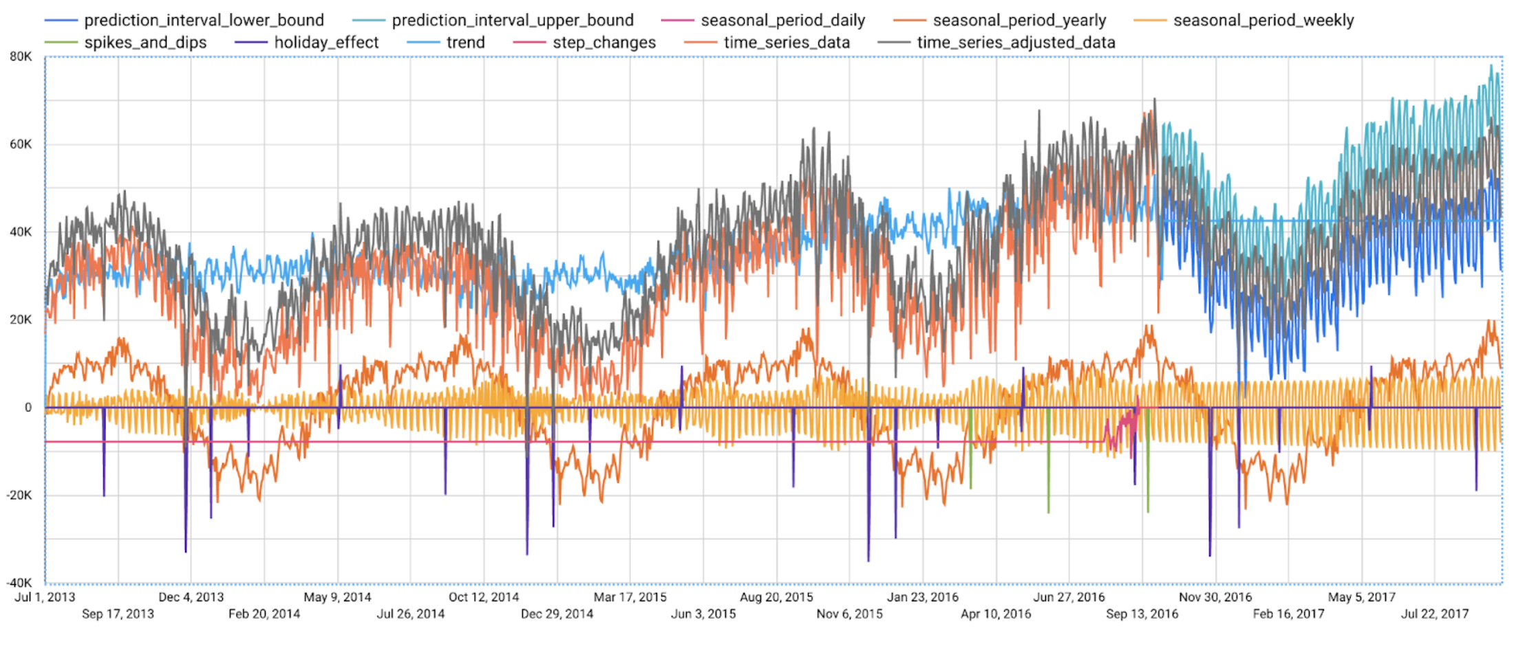
Compared to the previous figure which only shows the forecasting results, this figure shows much richer information to explain how the forecast is made.
First, it shows how the input time series is adjusted by removing the spikes and dips anomalies, and by compensating the level changes. That is:
time_series_adjusted_data = time_series_data - spikes_and_dips - step_changes
Second, it shows how the adjusted input time series is decomposed into different components such as both weekly and yearly seasonal components, holiday effect component and trend component. That is
time_series_adjusted_data = trend + seasonal_period_yearly + seasonal_period_weekly + holiday_effect + residual
Finally, it shows how these components are forecasted separately to compose the final forecasting results. That is:
time_series_data = trend + seasonal_period_yearly + seasonal_period_weekly + holiday_effect
For more information on these time series components, please see the documentation here.
Conclusion
With the GA of BigQuery Explainable AI, we hope you will now be able to interpret your machine learning models with ease.
Thanks to the BigQuery ML team, especially Lisa Yin, Jiashang Liu, Amir Hormati, Mingge Deng, Jerry Ye and Abhinav Khushraj. Also thanks to the Vertex Explainable AI team, especially David Pitman and Besim Avci.
How Digital Simulation of Physical Stores Helped e-Commerce Companies Replenish Stocks and Fulfil Online Orders at Scale in 2020

2974
Of your peers have already read this article.
3:00 Minutes
The most insightful time you'll spend today!
Editor’s note: We’re inviting partners from across our retail ecosystem to share stories, best practices, and tips and tricks on how they are helping retailers transform during a time that has seen tremendous change. The original version of this blog was published by Trax Retail in October 2021. Please enjoy this updated entry from our partner.

In 2020, we saw a massive leap in online grocery. Within a few weeks, the industry reached numbers that were unexpected for at least four more years. In a snap, what seemed like a relatively insignificant channel became one that grocery retailers simply couldn’t ignore and, what’s more, is likely to remain a norm.
Retailers trying to stay ahead of the curve have already started experimenting with methods like building warehouses and installing robots to fulfill the growing demand, but in-store picking has been and will continue to remain one of the primary methods of fulfilling online orders as it offers several advantages. First, it allows the use of existing infrastructure – large retailers already have geographically well-located outlets in major cities, which enables shorter lead time to delivery. Secondly, it allows retailers to stay flexible and move swiftly between in-store and online order fulfillment. And finally, it fits perfectly with the omnichannel approach to allow customers to shop wherever and however they want – click and collect, curbside pick-up, or inside brick-and-mortar stores.
How improving on-shelf availability helps ecommerce profitability

Despite its many advantages, in-store picking is expensive and affects profitability in an already competitive space since the cost of picking is directly tied with hourly labor fees. Moreover, with labor being a major challenge to obtain and retain, every minute spent picking counts. However, there is an easy way to keep costs down – optimizing the picking process by ensuring product availability and reducing the need for substitution.
An average of 8% of products are not available on-shelf in stores at any given time. As a result, pickers waste much of their time hunting for products that simply aren’t on the shelf or are misplaced, or spend time looking for substitutes, further increasing the time and cost for picking. In fact, grocery pickers often claim that out-of-stock (OOS) occurrences are the main reason that slows down the picking process. Without these factors, pick rates could be two times faster. Since picking accounts for 50% of the fulfillment cost, it has a substantial impact on the order’s bottom line and often makes the difference between a loss-making and a profitable basket.
Maintaining on-shelf availability for the thousands of products in every store has always been a significant problem to solve. The shift to online ordering has made the availability issue even more significant as the shelf is also now the fulfillment center for the majority of online orders. For e-commerce, out of stocks present two major issues for retailers. First, the impact of out-of-stock items is even more noticeable for online shoppers as they do not select their own substitutions. Additionally, out-of-stocks cause inefficiencies in the item fulfillment process, which is already a costly and margin-diluting practice for retailers. The good news is that through a partnership between Trax and Google Cloud, and the power of Google Cloud’s AI/ML capabilities, these challenges are addressed. The granular, real-time data at scale to enable picking efficiency and the data transparency to unlock a better shopping experience are now a reality which benefits both shoppers and store associates.
Trax and Google Cloud technology helps the bottom line
Trax and Google Cloud offer solutions that can help retailers improve on-shelf availability (OSA). Trax Retail Watch powered by Google Cloud uses computer vision (CV) and AI to create a digital version of the physical store in real-time and informs out-of-stocks so that retailers always have full visibility of items that are running low and can replenish them quickly. In turn, pickers are more likely to find everything they need quickly without facing the problem of missing products or having to look for substitutes. Trax Retail Watch also allows store associates to quickly spot any issues arising on shelves without having to physically walk down each aisle. From misplaced products to low stock, having full visibility means that shelf managers make more informed decisions, so that pickers face fewer obstacles, are aware of the true inventory, and significantly improve their pick rates. Faster picking means lower costs and ultimately, higher margins for online grocery orders.
With more e-commerce retailers crowding the online space, competition is tough. Want to know how frustrated e-commerce shoppers are about on-shelf availability? Trax uncovered this problem through an in-depth consumer study. Learn how to address shopper happiness while driving more profitable fulfillment and stay on the leaderboard with this Trax and Google Cloud whitepaper: Winning the online grocery race.
4542
Of your peers have already watched this video.
31:00 Minutes
The most insightful time you'll spend today!
How Google Secures its Data Centers: Watch Video
Security is in the DNA of Google Cloud’s dozens of data centers, complex network and workloads scattered the globe. Take a tour to the nucleus of data center’s six layers of physical security designed to keep unauthorized access at bay, and also learn about Google Cloud’s security fundamentals to leverage the same philosophy on Google Cloud. Watch now!
Master AI Prompt Engineering with 6 Proven Tips

1042
Of your peers have already read this article.
2:30 Minutes
The most insightful time you'll spend today!
As AI-powered tools become increasingly prevalent, prompt engineering is becoming a skill that developers need to master. Large language models (LLMs) and other generative foundation models require contextual, specific, and tailored natural language instructions to generate the desired output. This means that developers need to write prompts that are clear, concise, and informative.
In this blog, we will explore six best practices that will make you a more efficient prompt engineer. By following our advice, you can begin creating more personalized, accurate, and contextually aware applications. So let’s get started!
Tip #1: Know the model’s strengths and weaknesses
As AI models evolve and become more complex, it is essential for developers to comprehend their capabilities and limitations. Understanding these strengths and weaknesses can help you, as a developer, avoid making mistakes and create safer, more reliable applications.
For example, an AI model that is trained to recognize images of blueberries may not be able to recognize images of strawberries. Why? Because the model was only trained on a dataset of blueberry images. If a developer uses this model to build an application that is supposed to recognize both blueberries and strawberries, the application would likely make mistakes, leading to an ineffective outcome, and poor user experience.
It’s important to note that AI models have the ability to be biased. This is due to AI models being trained on data that is collected from the real world, and so it can reflect the inequitable power dynamics inherently rooted in our social hierarchy. If the data that is used to train an AI model is biased, then the model will also be biased. This can lead to problems if the model is used to make decisions that affect people by reinforcing societal biases. Addressing these biases is important to ensure that data is fair, promoting equality, and ensuring the responsibility of AI technology. Prompt engineers should be aware of training limitations or biases so they can craft prompts more effectively and understand what kind of prompting is even possible for a given model.

Tip #2: Be as specific as possible
AI models have the ability to comprehend a variety of prompts. For instance Google’s PaLM 2 can understand natural language prompts, multilingual text, and even programming codes like Python and JavaScript. Although AI models can be very knowledgeable, they are still imperfect, and have the ability to misinterpret prompts that are not specific enough. In order for AI models to navigate ambiguity, it is important to tailor your prompts specifically to your desired outcome.
Let’s say you would like your AI model to generate a recipe for 50 vegan blueberry muffins. If you prompt the model with “what is a recipe for blueberry muffins?”, the model does not know that you need to make 50 muffins. It is thus unlikely to list the larger volume of ingredients you’ll need or include tips to help you more efficiently bake such a large number of muffins. The model can only go off the context that is provided. A more effective prompt would be “I am hosting 50 guests. Generate a recipe for 50 blueberry muffins.” The model is more likely to generate a response that is relevant to your request and meets your specific requirements.
Tip #3: Utilize contextual prompts
Utilize contextual information in your prompts to help the model gain an in-depth understanding of your requests. Contextual prompts can include the specific task you want the model to perform, a replica of the output you’re looking for, or a persona to emulate, from a marketer or engineer to a high school teacher. Defining a tone and perspective for an AI model gives it a blueprint of the tone, style, and focused expertise you’re looking for to improve the quality, relevance, and effectiveness of your output.
In the case of the blueberry muffins, it is important to prompt the model using the context of the situation. The model might need more context than generating a recipe for 50 people. If it needs to be aware that the recipe must be vegan friendly, you might prompt the model by asking it to answer by emulating a skilled vegan chef.
By providing contextual prompts, you can help ensure that your AI interactions are as seamless and efficient as possible. The model will be able to more quickly understand your request and it will be able to generate more accurate and relevant responses.
Tip #4: Provide AI models with examples
When creating prompts for AI models, it is helpful to provide examples. This is because prompts act as instructions for the model, and examples can help the model to understand what you are asking for. Providing a prompt with an example looks something like this: “here are several recipes I like – create a new recipe based on the ones I provided.” The model can now understand the your ability and needs in order to make this pastry,
Tip #5: Experiment with prompts and personas
The way you construct your prompt impacts the model’s output. By creatively exploring different requests, you will soon have an understanding of how the model weighs its answers, and what happens when you interfuse your domain knowledge, expertise, and lived experience with the power of a multi-billion parameter large language model.
Try experimenting with different keywords, sentence structures, and prompt lengths to discover the perfect formula. Allow yourself to step into the shoes of various personas, from work personas such as “product engineer” or “customer service representatives,” to parental figures or celebrities such as your grandmother, a celebrity chef, and explore everything from cooking to coding!
By crafting unique, and innovative, requests replete with your expertise and experience, you can learn which prompts provide you with your ideal output. Further refining your prompts, known as ‘tuning,’ allows the model to have a greater understanding and framework for your next output.
Tip #6: Try chain-of-thought prompting
Chain of thought prompting is a technique for improving the reasoning capabilities of large language models (LLMs). It works by breaking down a complex problem into smaller steps, and then prompting the LLM to provide intermediate reasoning for each step. This helps the LLM to understand the problem more deeply, and to generate more accurate and informative answers. This will help you to understand the answer better and to make sure that the LLM is actually understanding the problem.
Conclusion
Prompt engineering is a skill that all workers, across industries and organizations, will need as AI-powered tools are becoming more prevalent. Remember to incorporate these five essential tips the next time you communicate with an AI model, so you can generate the accurate outputs that you desire. AI will forever continue to develop, constantly refining itself as we use it, so I encourage you to remember that learning, for mind and machine, is a never ending journey. Happy Prompting!

3738
Of your peers have already downloaded this article
8:30 Minutes
The most insightful time you'll spend today!
Automation and machine learning technologies are changing the way marketers drive results for their customers and brands. But there’s still a significant gap between those who are just talking about machine learning and those who are taking action.
For marketers looking to become leaders in their field, this is an exciting time. It’s a chance to make your mark, get ahead of competitors, and drive real results.
To explore this shifting landscape, Google partnered with the Massachusetts Institute of Technology Sloan Management Review (MIT SMR) to conduct a global survey and interview over a dozen executives and academics about their use of automation and machine learning technology and the results they’re seeing.
The survey’s findings show there are clear opportunities for marketers to get ahead of the pack.
While nearly three-quarters of the survey’s respondents believe their organization’s current goals would be better achieved with greater investment in machine learning and automation, only half the surveyed organizations have any incentives to make such investments.
View the survey results and unearth ways your organization can embrace machine learning and grasp the opportunity. Download the whitepaper now!
Simplifying Unstructured Data Analytics with BigQuery ML and Vertex AI: A Comprehensive Guide

1547
Of your peers have already read this article.
6:30 Minutes
The most insightful time you'll spend today!
Unstructured data such as images, speech and textual data can be notoriously difficult to manage, and even harder to analyze. The analysis of unstructured data includes use cases such as extracting text from images using OCR, sentiment analysis on customer reviews and simplifying translation for analytics. All of this data needs to be stored, managed and made available for machine learning.
The new BigQuery ML inference engine empowers practitioners to run inferences on unstructured data using pre-trained AI models. The results of these inferences can be analyzed to extract insights and improve decision making. This can all be done in BigQuery, using just a few lines of SQL.
In this blog, we’ll explore how the new BigQuery ML inference engine can be used to run inferences against unstructured data in BigQuery. We’ll demonstrate how to detect and translate text from movie poster images, and run sentiment analysis against movie reviews.
BigQuery ML’s new inference engine
Google Cloud is home to a suite of pre-trained AI models and APIs. The BigQuery ML inference engine can call these APIs and manage the responses on your behalf. All you have to do is define the model you want to use and run inferences against your data. All of this is done in BigQuery using SQL. The inference results are returned in JSON format and stored in BigQuery for analysis.
Why run your inferences in BigQuery?
Traditionally, working with AI models to run inferences required expertise in programming languages like Python. The ability to run inferences in BigQuery using just SQL can make generating insights from your data using AI simple and accessible. BigQuery is also serverless, so you can focus on analyzing your data without worrying about scalability and infrastructure.
The inference results are stored in BigQuery, which allows you to analyze your unstructured data immediately, without the need to move or copy your data. A key advantage here is that this analysis can also be joined with structured data stored in BigQuery, giving you the opportunity to deepen your insights. This can simplify data management and minimize the amount of data movement and duplication required.
Which models are supported?
For now, the BigQuery ML inference engine can be used with these pre-trained Vertex AI models:
- Vision AI API: This model can be used to extract features from images managed by BigQuery Object Tables and stored on Cloud Storage. For example, Vision AI can detect and classify objects, or read handwritten text.
- Translation AI API: This model can be used to translate text in BigQuery tables into over one hundred languages.
- Natural Language Processing API: This model can be used to derive meaning from textual data stored in BigQuery tables. For example, features like sentiment analysis can be used to determine whether the emotional tone of text is positive or negative.
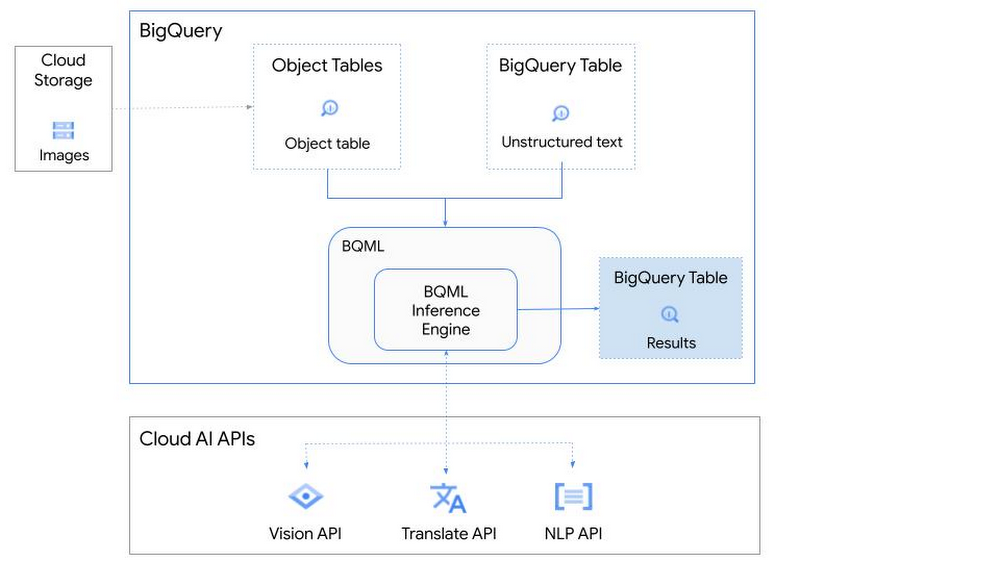
So, how does this work in practice? Let’s look at an example using images of movie posters

- We will define our pre-trained models for Vision AI, Translation AI and NLP AI in BigQuery ML.
- We’ll then use Vision AI to detect the text from some classic movie posters images.
- Next, we’ll use Translation AI to detect any foreign posters and translate them to a language of our choosing – English in this case.
- Finally, we’ll combine our unstructured data with structured data in BigQuery.
We’ll use the extracted movie titles from our movie posters to look up the viewer reviews from the BigQuery IMDB public dataset. We can then run sentiment analysis against these reviews using NLP AI.
Note: The BigQuery ML inference engine is currently in Preview. You will need to complete this enrollment form to have your project allowlisted for use with the BQML Inference Engine.
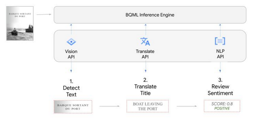
We’ll give examples of the BigQuery SQL needed to define your models and run your inferences. You’ll want to check out our notebook for a detailed guide on how to get this up and running in your Google Cloud project.
1. Define your AI Models in BigQuery
You will need to enable the APIs listed below, and also create a Cloud resource connection to enable BigQuery to interact with these services.
| API | Model Name |
| Vision AI API | Cloud_ai_vision_v1 |
| Translation AI API | Cloud_ai_translate_v3 |
| NLP AI API | Cloud_ai_natural_language_v1 |
You can then run the CREATE MODEL query for each AI service to create your pretrained models, replacing the model_name as required.
CREATE OR REPLACE MODEL
`{PROJECT_ID}.{DATASET_ID}.{VISION_MODEL_NAME}`
REMOTE WITH
CONNECTION `{PROJECT_ID}.{REGION}.{CONN_NAME}`
OPTIONS ( remote_service_type = '<model_name>' );
2. Use the Vision AI API to detect text in images stored in Cloud Storage
You will need to create an object table for your images in Cloud Storage. This read-only object table provides metadata for images stored in Cloud Storage:
CREATE OR REPLACE EXTERNAL TABLE
`{PROJECT_ID}.{DATASET_ID}.{OBJECT_TABLE_NAME}`
WITH
CONNECTION `{REGION}.{CONN_NAME}`
OPTIONS (object_metadata = 'SIMPLE', uris = ['{BUCKET_LOCATION}/*']);
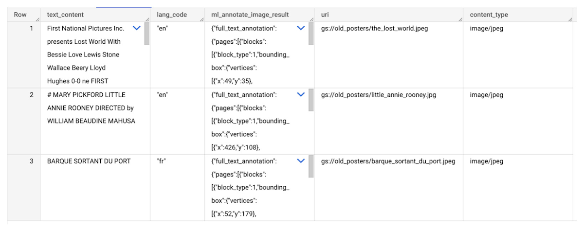
To detect the text from our posters, you can then use ML.ANNOTATE_IMAGE and specify the text_detection feature.
SELECT
       ml_annotate_image_result.full_text_annotation.text AS text_content,
       *
FROM
       ML.ANNOTATE_IMAGE(
         MODEL `{PROJECT_ID}.{DATASET_ID}.{VISION_MODEL_NAME}`,
         TABLE `{DATASET_ID}.{OBJECT_TABLE_NAME}`,
         STRUCT(['TEXT_DETECTION'] AS vision_features));
A JSON response will be returned to BigQuery that includes the text content and language code of the text. You can parse the JSON to a scalar result using the dot annotation highlighted above.

3. Use the Translation AI API to translate foreign movie titles
ML.TRANSLATE can now be used to translate the foreign titles we’ve extracted from our images into English. You just need to specify the target language and the table of the movie posters for translation:
SELECT
text_content,
STRING(ml_translate_result.translations[0].detected_language_code)
as original_language,
STRING(ml_translate_result.translations[0].translated_text)
as translated_title
FROM
  ML.TRANSLATE(
MODEL `{PROJECT_ID}.{DATASET_ID}.{TRANSLATE_MODEL_NAME}`,
TABLE `{DATASET_ID}.image_results`,
STRUCT('TRANSLATE_TEXT' as translate_mode, "en" as target_language_code));
Note: The table column with the text you want to translate must be named text_content:
The table of results will include json that can be parsed to extract both the original language and the translated text. In this case, the model has detected that title text is in French and has translated it to English:

4. Finally, use natural language processing (NLP) to run sentiment analysis against movie reviews
You can easily join inference results from your unstructured data with other BigQuery datasets to bolster your analysis. For example, we can now join the movie titles we extracted from our posters with thousands of movie reviews stored in BigQuery’s IMDB public dataset `bigquery-public-data.imdb.reviews`.
You can use ML.UNDERSTAND_TEXT with the analyze_sentiment feature to run sentiment analysis against some of these reviews to determine whether they are positive or negative:
SELECT
   primary_title, start_year, text_content AS review,
   FLOAT64(ml_understand_text_result.document_sentiment.score) AS score,
   FLOAT64(ml_understand_text_result.document_sentiment.magnitude) AS magnitude,
FROM
   ML.UNDERSTAND_TEXT(
     MODEL `{PROJECT_ID}.{DATASET_ID}.{NLP_MODEL_NAME}`,
           (
           SELECT
             primary_title, start_year, review AS text_content
           FROM
             `bigquery-public-data.imdb.title_basics` titles
           JOIN
             `bigquery-public-data.imdb.reviews` reviews
           ON
             reviews.movie_id = titles.tconst
           WHERE
             UPPER(titles.primary_title) = 'THE LOST WORLD' AND
             start_year = 1925
           ),
      STRUCT("analyze_sentiment" AS nlu_option)) ;
Note: The table column with the text you want to analyze must be named text_content:
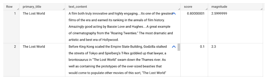
The JSON response will include a score and magnitude. The score indicates the overall emotion of the text while the magnitude indicates how much emotional content is present:
So, how did the Lost World compare with other movies that year?
To wrap up, we’ll compare the average review score of the 1925 Lost World movie to other movies released that year to see which was more popular. This can be done using familiar SQL analysis:
SELECT
 primary_title, start_year,
 AVG(FLOAT64(ml_understand_text_result.document_sentiment.score))AS av_score,
 AVG(FLOAT64(ml_understand_text_result.document_sentiment.magnitude)) AS av_magnitude
FROM
 ML.UNDERSTAND_TEXT(
   MODEL `{PROJECT_ID}.{DATASET_ID}.{NLP_MODEL_NAME}`,
         (
         SELECT
           primary_title, start_year, movie_id, review AS text_content
         FROM
           `bigquery-public-data.imdb.title_basics` titles
         JOIN
           `bigquery-public-data.imdb.reviews` reviews
         ON
           reviews.movie_id = titles.tconst
         WHERE
           start_year = 1925
         ),
   STRUCT("analyze_sentiment" AS nlu_option))
GROUP BY
   primary_title, start_year
ORDER BY
   av_score DESC;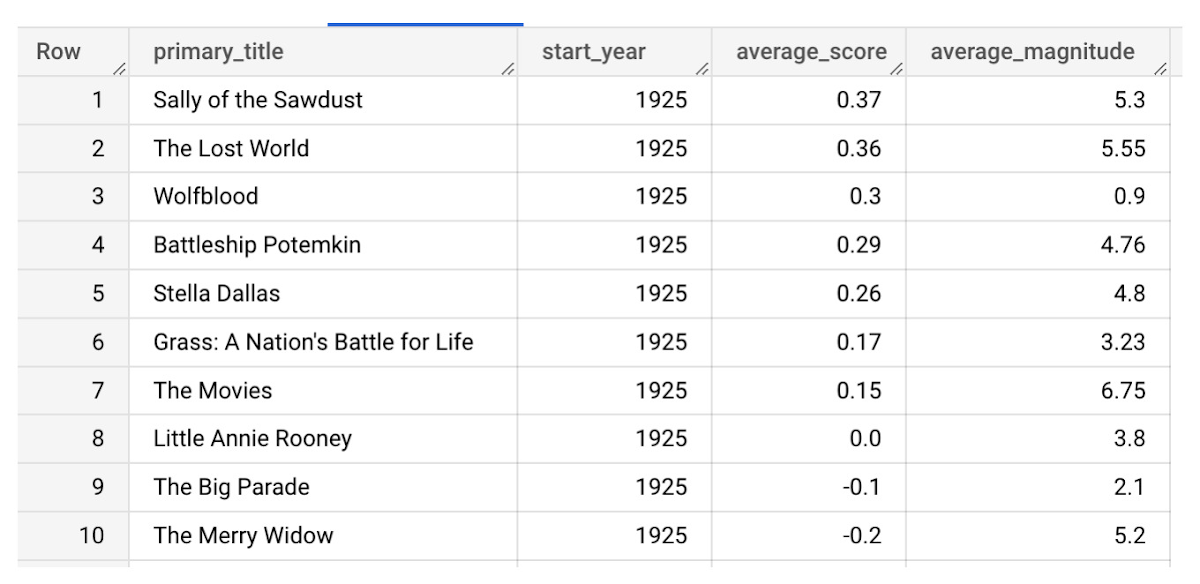
It looks like The Lost World narrowly missed out on the top spot to Sally of the Sawdust!
Want to learn more?
Check out our notebook for a step by step guide on using the BQML inference engine for unstructured data in Google Cloud. You can also check out our Cloud AI service table-valued functions overview page for more details. Curious about pricing? The BQML Pricing page gives a breakdown of how costs are applied across these services.
More Relevant Stories for Your Company

How Cleartrip.com is leveraging Google Cloud to survive the slump in the travel industry
With the novel coronavirus COVID-19 sweeping across continents and fatalities climbing every day, it was only a matter of time before countries closed their borders to contain its spread. In the wake of this decision, travel and tourism, the linchpins of many economies, were among the worst affected. According to

Hike: Processing Analytics Queries 20X Faster with Google Cloud Platform
After a seamless migration to Google Cloud Platform with CloudCover and Google Cloud Professional Services, Hike has reduced its costs by 20% and processed analytics queries 20 times faster than with its previous cloud provider. The business is also using AI and machine learning to enhance the experience provided by
Data Science Teams: A Practitioners Guide to MLOps
Across industries, DevOps and DataOps have been widely adopted as methodologies to improve quality and reduce the time to market of software engineering and data engineering initiatives. With the rapid growth in machine learning (ML) systems, similar approaches need to be developed in the context of ML engineering, which handle



Transitioning Kagglers to TPU with TF 2.x
Kaggle has, historically, become synonymous with machine learning competitions but it's much more than that. Kaggle is a data science platform. Over 5 million data scientists from all over the world come to Kaggle to not only not only participate in machine learning competitions but to learn data science build
