Editor’s note: Renault, the French automaker, embarked on a wholesale migration of its information systems—moving 70 applications to Google Cloud. Here’s how they migrated from Oracle databases to Cloud SQL for PostgreSQL.

The Renault Group, known for its iconic French cars has grown to include four complementary brands, and sold nearly 3 million vehicles in 2020. Following our company-wide strategic plan, “Renaulution,” we’ve shifted our focus over the past year from a car company integrating tech, to a tech company integrating cars that will develop software for our business. For the information systems group, that meant modernizing our entire portfolio and migrating 70 in-house applications (our quality and customer information systems) to Google Cloud. It was an ambitious project, but it’s paid off. In two years we migrated our Quality and Customer Satisfaction information systems applications, optimized our code, and cut costs thanks to managed database services. Compared to our on-premises infrastructure, using Google Cloud services and open-source technologies comes to roughly one dollar per user per year, which is significantly cheaper.

An ambitious journey to Google Cloud

We began our cloud journey in 2016 with digital projects integrating a new way of working and new technologies. These new technologies included those for agility at scale, data capabilities and CI/CD toolchain. Google Cloud stood out as the clear choice for its data capabilities. Not only are we using BigQuery and Dataflow to improve scaling and costs, but we are also now using fully managed database services like Cloud SQL for PostgreSQL. Data is a key asset for a modern car maker because it connects the car maker to the user, allows car makers to better understand usage and better informs what decisions we should make about our products and services. After we migrated our data lake to Google Cloud, it was a natural next step to move our front-end applications to Google Cloud so they would be easier to maintain and we could benefit from faster response times. This project was no small undertaking. For those 70 in-house applications (e.g. vehicle quality evaluation, statistical process control in plants, product issue management, survey analysis), for our information systems landscape, we had a range of technologies—including Oracle, MySQL, Java, IBM MQ, and CFT—with some applications created 20 years ago.

Champions spearhead each migration

Before we started the migration, we did a global analysis of the landscape to understand each application and its complexity. Then we planned a progressive approach, focusing on the smallest applications first such as those with a limited number of screens or with simple SQL queries, and saving the largest for last. Initially we used some automatic tools for the migration, but we learned very quickly nothing can replace the development team’s institutional knowledge. They served as our migration champions.

The apps go marching one by one

When we migrated our first few Oracle databases to Cloud SQL for PostgreSQL we tracked our learnings in an internal wiki to share common SQL patterns, which helped us speed up the process. For some applications, we simplified the architecture and took the opportunity to analyze and optimize SQL queries during the rework. We also used monitoring tools like Dynatrace and JavaMelody to ensure we improved the user experience.

The approach we developed was very successful—where database migration was initially seen as insurmountable, the entire migration project was completed in two years.

With on-premises applications it was hard for our developers to separate code performance from infrastructure limitations. So as part of our migration to Google Cloud, we optimized our applications with monitoring services. With these insights our team has more control over resources, which has reduced our maintenance and operations activity and resulted in faster, more stable applications. Plus, migrating to Cloud SQL has made it much easier for us to change our infrastructure as needed, add more power when necessary or even reduce our infrastructure size.

A new regime on Cloud SQL

Now that we’re running on Cloud SQL, we’ve improved performance even on large databases with many connected users. Thanks to built-in tools in the Google Cloud environment, we can now easily understand performance issues and quickly solve them. For example, we were able to reduce the duration of a heavy batch processing by a factor of three from nine to three hours. And we don’t have to wait for the installation of a new server, so our team can move faster. Beyond speed, we’ve also been able to cut costs. We optimized our code based on insights from monitoring tools, which not only enabled a more responsive application for the user, but it also reduced our costs because we’re not overprovisioned.

Learn more about the Renault Group and try out Cloud SQL today.

When you’re serving customers online, speed is essential for a good experience. As the amount of data in a database grows, queries that used to be fast can slow down.

For example, if a query has to scan every row because a table is missing an index, response times that were acceptable with a thousand rows can turn into multiple seconds of waiting once you have a million rows.

If this query is executed every time a user loads your web page, their browsing experience will slow to a crawl, causing user frustration. Slow queries can also impact automated jobs, causing them to time out before completion.

If there are too many of these slow queries executing at once, the database can even run out of connections, causing all new queries, slow or fast, to fail. 

The popular open-source databases MySQL and Google Cloud Platform‘s fully managed version, Cloud SQL for MySQL, include a feature to log slow queries, letting you find the cause, then optimize for better performance.

However, developers and database administrators typically only access this slow query log reactively, after users have seen the effects and escalated the performance degradation.

With Stackdriver Logging and Monitoring, you can stay ahead of the curve for database performance with automatic alerts when query latency goes over the threshold, and a monitoring dashboard that lets you quickly pinpoint the specific queries causing the slowdown.

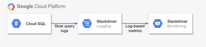
To get started, import MySQL’s slow query log into Stackdriver Logging.

Once the logs are in Stackdriver, it’s straightforward to set up logs-based metrics that can both count the number of slow queries over time, which is useful for setting up appropriate alerts, and also provide breakdowns by slow SQL statement, allowing speedy troubleshooting.

What’s more, this approach works equally well for managed databases in Cloud SQL for MySQL and for self-managed MySQL databases hosted on Compute Engine. 

For a step-by-step tutorial to set up slow query monitoring, check out Monitoring slow queries in MySQL with Stackdriver. For more ideas about what else you can accomplish with Stackdriver Logging, check out Design patterns for exporting Stackdriver Logging.

Editor’s note: Technology today lets companies of any size take on entire industries simply with an innovative business model plus digital distribution. Take Shine, a French startup whose platform helps freelancers manage their finances — and their administrative commitments. Here, Raphael Simon, Shine’s CTO and co-founder, talks about why Shine built a new bank on Google Cloud Platform, and in particular Cloud Spanner.

More and more people are deciding to take the plunge and start a freelance career. Some of them by choice, others out of necessity. One of their biggest pain points is dealing with administrative tasks.

In some countries, especially in Europe, the administrative burden of being a freelancer is similar to what a company of 10 or more people deals with. A freelancer doesn’t necessarily have the time or skills to manage all this paperwork. So we are building a new bank for freelancers from the ground up that helps automate administrative tasks associated with their business.

Shine’s banking services and financial tools make it as easy to work as a freelancer as it is to work for a larger company. We deal with administrative tasks on behalf of the freelancer so that he or she can focus on their job: finding and wowing clients.

Building our infrastructure 

As a new bank, we had the opportunity to build our infrastructure from the ground up. Designing an infrastructure and choosing a database presents tough decisions, especially in the financial services world. Financial institutions come under tremendous scrutiny to demonstrate stability and security. Even a tiny leak of banking data can have tremendous consequences both for the bank and its clients, and any service interruption can trigger a banking license to be suspended or a transaction to be declined.

At the same time, it’s vital for us to optimize our resources so we can maximize the time we spend developing user-facing features. In our first six months, we iterated and validated a prototype app using Firebase, and secured our seed funding round (one of the largest in Europe in 2017).

Based on our positive experience with Firebase, plus the ease-of-use and attractive pricing that Google Cloud offered, we decided to build our platform on Google Cloud Platform (GCP).

We were drawn to GCP because it has a simple, consistent interface that is easy to learn. We chose App Engine flexible environment with Google Cloud Endpoints for an auto-scaling microservices API. These helped us reduce the time, effort, and cost in terms of DevOps engineers, so we could invest more in developing features, while maintaining our agility.

We use Cloud Identity and Access Management (Cloud IAM) to help control developer access to critical parts of the application such as customer bank account data. It was quite a relief to lean on a reliable partner like Google Cloud for this.

Database decisions 

Next came time to choose a database. Shine lives at the financial heart of our customers’ businesses and provides guidance on things like accounting and tax declaration. The app calculates the VAT for each invoice and forecasts the charges they must pay each quarter.

Due to the sensitivity of our customers’ data, the stakes are high. We pay careful attention to data integrity and availability and only a relational database with support for ACID transactions (Atomicity, Consistency, Isolation, Durability) can meet this requirement.

At the same time, we wanted to focus on the app and user experience, not on database administration or scalability issues. We’re trying to build the best possible product for our users, and administering a database has no direct value for our customers. In other words, we wanted a managed service.

Cloud Spanner combines a globally distributed relational database service with ACID transactions, industry-standard SQL semantics, horizontal scaling, and high availability. Cloud Spanner provided additional security, high-availability, and disaster recovery features out-of-the-box that would have taken months for us to implement on our own. Oh, and no need to worry about performance — Cloud Spanner is fast. Indeed, Cloud Spanner has been a real asset to the project, from the ease-of-use of creating an instance to scaling the database.

Cloud Spanner pro tips 

We began working with Cloud Spanner and have learned a lot along the way. Here are some technical notes about our deployment and some best practices that may be useful to you down the road:

• Cloud Spanner allows us to change a schema in production without downtime. We always use a NOT NULL constraint, because we generally think that using NULL leads to more errors in application code. We always use a default value when we create an entity through our APIs and we use Cloud Dataflow to set values when we change a schema (e.g., adding a field to an entity). 
• With microservices, it’s generally a good practice to make sure every service has its own database to ensure data isolation between the different services. However, we adopted a slightly different strategy to optimize our use of Cloud Spanner. We have an instance on which there are three databases — one for production, one for staging and one for testing our continuous integration (CI) pipeline. Each service has one or more interleaved tables that are isolated from others services’ tables (we do not use foreign-keys between tables from different services). This way our microservices data are not tightly “coupled”. 
• We created an internal query service that performs read-only queries to Cloud Spanner to generate a dashboard or do complex queries for analytics. It is the only service where we allow joins between tables across services. 
• We take advantage of Cloud Spanner’s scalability, and thus don’t delete any data that could one day be useful and/or profitable. 
• We store all of our business logs on Cloud Spanner, for example connection attempts to the application. We append the ‘-Logs’ suffix to them. 
• When possible, we always create an interleave. 

 In short, implementing Cloud Spanner has been a good choice for Shine:

• It’s saved us weeks, if not months, of coding. 
• We feel we can rely on it since it’s been battle-tested by Google. 
• We can focus on building a disruptive financial services product for freelancers and SMBs.

And because Cloud Spanner is fully managed and horizontally scalable, we don’t have to worry about hardware, security patches, scaling, database sharding, or the possibility of a long and risky database migration in the future. We are confident Cloud Spanner will grow with our business, particularly as we expand regionally and globally. I strongly recommend Cloud Spanner to any company looking for a complete database solution for business-critical, sensitive, and scalable data.

Explainable AI (XAI) helps you understand and interpret how your machine learning models make decisions. We’re excited to announce that BigQuery Explainable AI is now generally available (GA). BigQuery is the data warehouse that supports explainable AI in a most comprehensive way w.r.t both XAI methodology and model types. It does this at BigQuery scale, enabling millions of explanations within seconds with a single SQL query.

Why is Explainable AI so important? To demystify the inner workings of machine learning models, Explainable AI is quickly becoming an essential and growing need for businesses as they continue to invest in AI and ML. With 76% of enterprises now prioritizing artificial intelligence (AI) and machine learning (ML) over other initiatives in 2021 IT budgets, the majority of CEOs (82%) believe that AI-based decisions must be explainable to be trusted according to a PwC survey.

While the focus of this blogpost is on BigQuery Explainable AI, Google Cloud provides a variety of tools and frameworks to help you interpret models outside of BigQuery, such as with Vertex Explainable AI, which includes AutoML Tables, AutoML Vision, and custom-trained models.

So how does Explainable AI in BigQuery work exactly? And how might you use it in practice? 

Two types of Explainable AI: global and local explainability

When it comes to Explainable AI, the first thing to note is that there are two main types of explainability as they relate to the features used to train the ML model: global explainability and local explainability.

Imagine that you have a ML model that predicts housing price (as a dollar amount), based on three features: (1) number of bedrooms, (2) distance to the nearest city center, and (3) construction date.

Global explainability (a.k.a. global feature importance) describes the features’ overall influence on the model and helps you understand if a feature had a greater influence than other features over the model’s predictions. For example, global explainability can reveal that the number of bedrooms and distance to city center typically has a much stronger influence than the construction date on predicting housing prices. Global explainability is especially useful if you have hundreds or thousands of features and you want to determine which features are the most important contributors to your model. You may also consider using global explainability as a way to identify and prune less important features to improve the generalizability of their models.

Local explainability (a.k.a. feature attributions) describes the breakdown of how each feature contributes towards a specific prediction. For example, if the model predicts that house ID#1001 has a predicted price of $230,000, local explainability would describe a baseline amount (e.g. $50,000) and how each of the features contributes on top of the baseline towards the predicted price. For example, the model may say that on top of the baseline of $50,000, having 3 bedrooms contributed an additional $50,000, close proximity to the city center added $100,000, and construction date of 2010 added $30,000, for a total predicted price of $230,000. In essence, understanding the exact contribution of each feature used by the model to make each prediction is the main purpose of local explainability.

What ML models does BigQuery Explainable AI apply to?

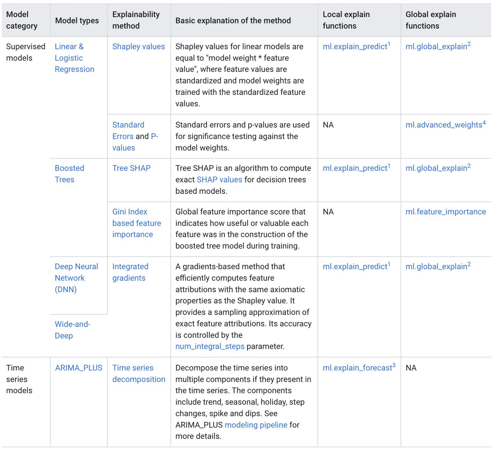
BigQuery Explainable AI applies to a variety of models, including supervised learning models for IID data and time series models. The documentation for BigQuery Explainable AI provides an overview of the different ways of applying explainability per model. Note that each explainability method has its own way of calculation (e.g. Shapley values), which are covered more in-depth in the documentation.

Examples with BigQuery Explainable AI

In this next section, we will show three examples of how to use BigQuery Explainable AI in different ML applications: 

• regression 
• classification
• time-series forecasting

Regression models with BigQuery Explainable AI

Let’s use a boosted tree regression model to predict how much a taxi cab driver will receive in tips for a taxi ride, based on features such as number of passengers, payment type, total payment and trip distance. Then let’s use BigQuery Explainable AI to help us understand how the model made the predictions in terms of global explainability (which features were most important?) and local explainability (how did the model arrive at each prediction?).

The taxi trips dataset comes from the BigQuery public datasets and is publicly available in the table: bigquery-public-data.new_york_taxi_trips.tlc_yellow_trips_2018. 

First, you can train a boosted tree regression model.

  CREATE OR REPLACE MODEL bqml_tutorial.taxi_tip_regression_model
OPTIONS (model_type='boosted_tree_regressor',
         input_label_cols=['tip_amount'],
         max_iterations = 50,
         tree_method = 'HIST',
         subsample = 0.85,
         enable_global_explain = TRUE
) AS
SELECT
  vendor_id,
  passenger_count,
  trip_distance,
  rate_code,
  payment_type,
  total_amount,
  tip_amount
FROM
  `bigquery-public-data.new_york_taxi_trips.tlc_yellow_trips_2018`
WHERE tip_amount >= 0
LIMIT 1000000

Now let’s do a prediction using ML.PREDICT, which is the standard way in BigQuery ML to make predictions without explainability.

  SELECT *
FROM
ML.PREDICT(MODEL bqml_tutorial.taxi_tip_regression_model,
 (
 SELECT
   "0" AS vendor_id,
   1 AS passenger_count,
   CAST(5.85 AS NUMERIC) AS trip_distance,
   "0" AS rate_code,
   "0" AS payment_type,
   CAST(55.56 AS NUMERIC) AS total_amount))

But you might wonder—how did the model generate this prediction of ~11.077?

BigQuery Explainable AI can help us answer this question. Instead of using ML.PREDICT, you use ML.EXPLAIN_PREDICT with an additional optional parameter top_k_features. ML.EXPLAIN_PREDICT extends the capabilities of ML.PREDICT by outputting several additional columns that explain how each feature contributes to the predicted value. In fact, since ML.EXPLAIN_PREDICT includes all the output from ML.PREDICT anyway, you may want to consider using ML.EXPLAIN_PREDICT every time instead.

  SELECT *
FROM
ML.EXPLAIN_PREDICT(MODEL bqml_tutorial.taxi_tip_regression_model,
 (
 SELECT
   "0" AS vendor_id,
   1 AS passenger_count,
   CAST(5.85 AS NUMERIC) AS trip_distance,
   "0" AS rate_code,
   "0" AS payment_type,
   CAST(55.56 AS NUMERIC) AS total_amount),
 STRUCT(6 AS top_k_features))

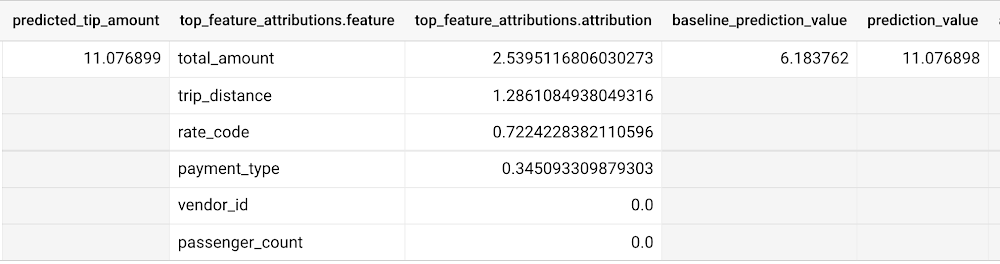
The way to interpret these columns is:

Σfeature_attributions + baseline_prediction_value = prediction_value

Let’s break this down. The prediction_value is ~11.077, which is simply the predicted_tip_amount. The baseline_prediction_value is ~6.184, which is the tip amount for an average instance. top_feature_attributions indicates how much each of the features contributes towards the prediction value. For example, total_amount contributes ~2.540 to the predicted_tip_amount. 

ML.EXPLAIN_PREDICT provides local feature explainability for regression models. For global feature importance, see the documentation for ML.GLOBAL_EXPLAIN.

Classification models with BigQuery Explainable AI

Let’s use a logistic regression model to show you an example of BigQuery Explainable AI with classification models. We can use the same public dataset as before: bigquery-public-data.new_york_taxi_trips.tlc_yellow_trips_2018.

Train a logistic regression model to predict the bracket of the percentage of the tip amount out of the taxi bill.

  CREATE OR REPLACE MODEL bqml_tutorial.taxi_tip_classification_model
OPTIONS
 (model_type='logistic_reg',
  input_label_cols=['tip_bucket'],
  enable_global_explain=true
) AS
SELECT
  vendor_id,
  passenger_count,
  trip_distance,
  rate_code,
  payment_type,
  total_amount,
  CASE
    WHEN tip_amount > total_amount*0.20 THEN '20% or more'
    WHEN tip_amount > total_amount*0.15 THEN '15% to 20%'
    WHEN tip_amount > total_amount*0.10 THEN '10% to 15%'
  ELSE '10% or less'
  END AS tip_bucket
FROM
  `bigquery-public-data.new_york_taxi_trips.tlc_yellow_trips_2018`
WHERE tip_amount >= 0
LIMIT 1000000

Next, you can run ML.EXPLAIN_PREDICT to get both the classification results and the additional information for local feature explainability. For global explainability, you can use ML.GLOBAL_EXPLAIN. Again, since ML.EXPLAIN_PREDICT includes all the output from ML.PREDICT anyway, you may want to consider using ML.EXPLAIN_PREDICT every time instead.

  SELECT *
FROM
ML.EXPLAIN_PREDICT(MODEL bqml_tutorial.taxi_tip_classification_model,
 (
 SELECT
   "0" AS vendor_id,
   1 AS passenger_count,
   CAST(5.85 AS NUMERIC) AS trip_distance,
   "0" AS rate_code,
   "0" AS payment_type,
   CAST(55.56 AS NUMERIC) AS total_amount),
 STRUCT(6 AS top_k_features))

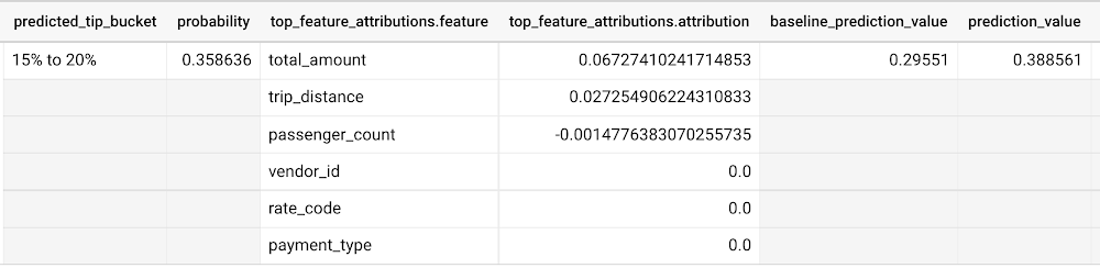
Similar to the regression example earlier, the formula is used to derive the prediction_value:

Σfeature_attributions + baseline_prediction_value = prediction_value

As you can see in the screenshot above, the baseline_prediction_value is ~0.296. total_amount is the most important feature in making this specific prediction, contributing ~0.067 to the prediction_value, though followed by trip_distance. The feature passenger_count contributes negatively to prediction_value by -0.0015. The features vendor_id, rate_code, and payment_type did not seem to contribute much to the prediction_value.

You may wonder why the prediction_value of ~0.389 doesn’t equal the probability value of  ~0.359. The reason is that unlike for regression models, for classification models, prediction_value is not a probability score. Instead, prediction_value is the logit value (i.e., log-odds) for the predicted class, which you could separately convert to probabilities by applying the softmax transformation to the logit values. For example, a three-class classification has a log-odds output of [2.446, -2.021, -2.190]. After applying the softmax transformation, the probability of these class predictions is [0.9905, 0.0056, 0.0038].

Time-series forecasting models with BigQuery Explainable AI

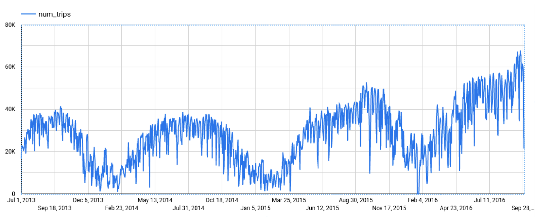
Explainable AI for forecasting provides more interpretability into how the forecasting model came to its predictions. Let’s go through an example of forecasting the number of bike trips in NYC using the new_york.citibike_trips public data in BigQuery.

You can train a time-series model ARIMA_PLUS:

  CREATE OR REPLACE MODEL bqml_tutorial.nyc_citibike_arima_model
OPTIONS
  (model_type = 'ARIMA_PLUS',
   time_series_timestamp_col = 'date',
   time_series_data_col = 'num_trips',
   holiday_region = 'US'
  ) AS
SELECT
   EXTRACT(DATE from starttime) AS date,
   COUNT(*) AS num_trips
FROM
  `bigquery-public-data.new_york.citibike_trips`
GROUP BY date

Next, you can first try forecasting without explainability using ML.FORECAST:
SELECT
  *
FROM
  ML.FORECAST(MODEL bqml_tutorial.nyc_citibike_arima_model,
              STRUCT(365 AS horizon, 0.9 AS confidence_level))

This function outputs the forecasted values and the prediction interval. Plotting it in addition to the input time series gives the following figure.

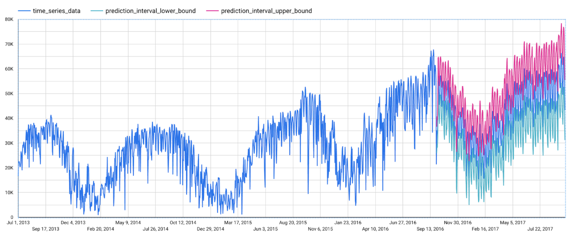
But how does the forecasting model arrive at its predictions? Explainability is especially important if the model ever generates unexpected results.

With ML.EXPLAIN_FORECAST, BigQuery Explainable AI provides extra transparency into the seasonality, trend, holiday effects, level (step) changes, and spikes and dips outlier removal. In fact, since ML.EXPLAIN_FORECAST includes all the output from ML.FORECAST anyway, you may want to consider using ML.EXPLAIN_FORECAST every time instead.

  SELECT
  *
FROM
  ML.EXPLAIN_FORECAST(MODEL bqml_tutorial.nyc_citibike_arima_model,
                      STRUCT(365 AS horizon, 0.9 AS confidence_level))

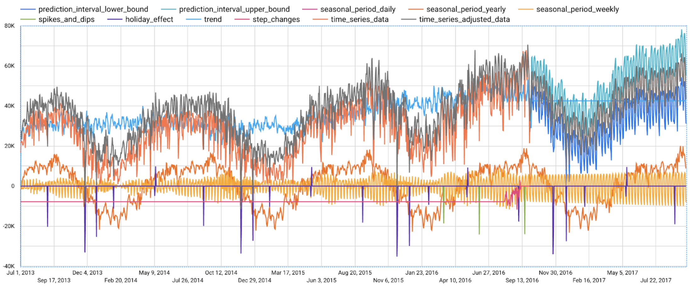
Compared to the previous figure which only shows the forecasting results, this figure shows much richer information to explain how the forecast is made.  

First, it shows how the input time series is adjusted by removing the spikes and dips anomalies, and by compensating the level changes. That is:

time_series_adjusted_data = time_series_data - spikes_and_dips - step_changes

Second, it shows how the adjusted input time series is decomposed into different components such as both weekly and yearly seasonal components, holiday effect component and trend component. That is

time_series_adjusted_data = trend + seasonal_period_yearly + seasonal_period_weekly + holiday_effect + residual

Finally, it shows how these components are forecasted separately to compose the final forecasting results. That is:

time_series_data = trend + seasonal_period_yearly + seasonal_period_weekly + holiday_effect

For more information on these time series components, please see the documentation here.

Conclusion

With the GA of BigQuery Explainable AI, we hope you will now be able to interpret your machine learning models with ease. 

Thanks to the BigQuery ML team, especially Lisa Yin, Jiashang Liu, Amir Hormati, Mingge Deng, Jerry Ye and Abhinav Khushraj. Also thanks to the Vertex Explainable AI team, especially David Pitman and Besim Avci.