





Google Cloud’s Data Analytics May Recap

6919
Of your peers have already read this article.
5:00 Minutes
The most insightful time you'll spend today!
May was a very busy month for data analytics product innovation. If you didn’t have the chance to attend our inaugural Data Cloud Summit, video replays of all our sessions are now available so feel free to watch them at your own pace.
In this blog, I’d like to share some background behind the innovations we released in May, why we built them the way we did, and the type of value they can bring your company and your team.
But first, a huge thank you!
This week, we had the honor to announce that Google has been named a Leader in The Forrester Wave™: Streaming Analytics, Q2 2021 report. Forrester gave Dataflow a score of 5 out of 5 across 12 different criteria, stating: “Google Cloud Dataflow has strengths in data sequencing, advanced analytics, performance, and high-availability”.
Google has more than a decade of experience in building real-time and internet-scale systems for its own needs, and we are excited to see that our ability to provide customers with a reliable, scalable, and performant platform is bearing fruit.
This announcement comes on the back of the release of The Forrester Wave™: Cloud Data Warehouse, Q1 2021 report, which also named Google Cloud as a Leader.
We couldn’t be more excited about the recognition and appreciate all your feedback and trust in the work that we do to support your goal in accelerating data-powered innovation.
Innovation galore
Your feedback and your passion is the fuel that drives our ambition to deliver more and better services to you. That’s why, this year, we didn’t want to wait until Google Cloud Next to share some great products we have been working on. On May 26, our team announced a slew of new products, services and programs. Watch a quick summary below:
https://youtube.com/watch?v=DG1mOPMXJvw%3Fenablejsapi%3D1%26
Meeting you where you are
An important design principle behind all of our services is “meeting you where you are”. This means we aim to provide you with the tools and software you need to innovate on your own terms. Here are three new services that will help you do just that:
Datastream
Datastream, our new serverless change data capture (CDC) and replication service, allows your company to synchronize data across heterogeneous databases, storage systems, and applications reliably and with minimal latency to support real-time analytics, database replication, and event-driven architectures. Datastream delivers change streams from Oracle and MySQL databases into Google Cloud services such as BigQuery, Cloud SQL, Cloud Storage, and Cloud Spanner, saving time and resources while ensuring your data is accurate and up-to-date.
- Under the hood, Datastream reads CDC events (inserts, updates, and deletes) from source databases, and writes those events with minimal latency to a data destination. It leverages the fact that each database source has its own CDC log—binlog for MySQL and LogMiner for Oracle—which it uses for its own internal replication and consistency purposes.
- Datastream integrates with purpose-built and extensible Dataflow templates to pull the change streams written to Cloud Storage, and create up-to-date replicated tables in BigQuery for analytics. It also leverages Dataflow templates to replicate and synchronize databases into Cloud SQL or Cloud Spanner for database migrations and hybrid cloud configurations.
- Datastream also powers a Google-native Oracle connector in Cloud Data Fusion’s new replication feature for easy ETL/ELT pipelining. By delivering change streams directly into Cloud Storage, customers can leverage Datastream to implement modern, event-driven architectures.
Looker and BigQuery Omni on Microsoft Azure
Research on multi cloud adoption is unequivocal — 92% of businesses in 2021 report having a multi cloud strategy. We want to continue supporting your choice by providing the flexibility you need to see your strategy through.
- This past month, we introduced Looker, hosted on Microsoft Azure. For the first time, you can now choose Azure, Google Cloud, or AWS for your Looker instance. You can also self-host your Looker instance on-premises.
- We also introduced BigQuery Omni for Azure, which along with last year’s introduction of BigQuery Omni for AWS, will help you access and securely analyze data across Google Cloud, AWS, and Azure.
The cost of moving data between cloud providers isn’t sustainable for many, and it’s still difficult to seamlessly work across clouds. BigQuery Omni represents a new way of analyzing data stored in multiple public clouds, which is made possible by BigQuery’s separation of compute and storage. By decoupling these two, BigQuery provides scalable storage that can reside in Google Cloud or other public clouds, and stateless resilient compute that executes standard SQL queries.
- Unlike competitors, BigQuery Omni doesn’t require you to move or copy your data from one public cloud to another, where you might incur egress costs. You also benefit from the same BigQuery interface on Google Cloud, enabling you to query data stored in Google Cloud, AWS, and Azure without any cross-cloud movement or copies of data.
- BigQuery Omni’s query engine runs the necessary compute on clusters in the same region where your data resides. For example, you can query Google Analytics 360 Ads data stored in Google Cloud and query logs data from your ecommerce platform and applications that are stored in AWS S3 and/or Microsoft Azure.
Then, using Looker, you can build a dashboard that allows you to visualize your audience behavior and purchases alongside your advertising spend.
Dataplex
We understand that most organizations still struggle to make high-quality data easily discoverable and accessible for analytics, across multiple silos, to a growing number of people and tools within their organization.
They are often forced to make tradeoffs. For instance, moving and duplicating data across silos to enable diverse analytics use cases or leaving their data distributed but limiting the agility of decisions.
- Dataplex provides an intelligent data fabric that enables you to centrally manage, monitor, and govern your data across data lakes, data warehouses, and data marts, while also ensuring data is securely accessible to a variety of analytics and data science tools.
- One of the core tenets of Dataplex is letting you organize and manage your data in a way that makes sense for your business, without data movement or duplication. For that, we provide logical constructs like lakes, data zones, and assets. These constructs enable you to abstract away the underlying storage systems and become the foundation for setting policies around data access, security, lifecycle management, and so on.
- For example, you can create a lake per department within your organization (e.g. Retail, Sales, Finance, etc.) and create data zones that map to data readiness and usage (e.g. landing, raw, curated_data_analytics, curated_data_science, etc.).
Once you have your lakes and zones setup, you can attach data to these zones as assets. You can add data from different types of storage (e.g. GCS Bucket and BigQuery dataset) under the same zone. You can also attach data across multiple projects under the same zone. You can ingest data into your lakes and zones using the tools of your choice, including services such as Dataflow, Data Fusion, Dataproc, Pub/Sub, or choose from one of our partner products. Dataplex comes with built-in 1-click templates for common data management tasks.
To find out more about Dataplex, head to cloud.google.com/dataplex or watch the video below:
https://youtube.com/watch?v=bbFeAt7cw1g%3Fenablejsapi%3D1%26
Helping you innovate everyday
Sharing data is hard. Traditional data sharing techniques use batch data pipelines that are expensive to run, create late arriving data, and can break with any changes to the source data. These techniques also create multiple copies of data, which brings unnecessary costs and can bypass data governance processes. They also fail to offer features for data monetization, such as managing subscriptions and entitlements. Altogether, these challenges mean that organizations are unable to realize the full potential of transforming their business with shared data.
Analytics Hub
To address these limitations, we are introducing Analytics Hub, a new fully managed service that helps organizations unlock the value of data sharing, leading to new insights and increased business value.
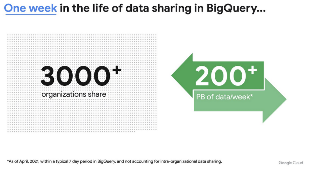
This new service is built on the tremendous experience and feedback we have received over the years. For example, BigQuery has had cross-organizational, in-place data sharing capabilities since its inception in 2010—and the functionality is very popular. Over a 7-day period in April, we had over 3,000 different organizations sharing over 200 petabytes of data. These numbers don’t include data sharing between departments within the same organization.
Analytics Hub takes sharing to the next level, making it easy for you to publish, discover, and subscribe to valuable datasets that you can combine with your own data to derive unique insights.
This includes:
- Shared datasets: As a data publisher, you create shared datasets that contain the views of data that you want to deliver to your subscribers. Data subscribers can search through the datasets that are available across all exchanges for which they have access and subscribe to relevant datasets. In addition, the publisher can track subscribers, disable subscriptions, and see aggregated usage information for the shared data.
- Curated, self-service data exchanges: Exchanges are collections used to organize and secure shared datasets. By default, exchanges are completely private, but granular roles and permissions make it easy to deliver data to the right audience—whether internal or public.
This is just the beginning for Analytics Hub. Please sign up for the preview, which is scheduled to be available in the third quarter of 2021.
Dataflow Prime
At Google Cloud, we have the great privilege of working with some of the most innovative organizations in the world. And this work provides us with a unique perspective into the future of big data processing. Dataflow Prime is a new platform based on a serverless, no-ops, and auto-tuning architecture that brings unparalleled resource utilization and radical operational simplicity to big data processing. This new service introduces a large number of exciting capabilities but I’d like to highlight three key aspects of the product:
- Vertical Autoscaling: Dataflow Prime dynamically adjusts the compute capacity allocated to each worker based on utilization, detecting when jobs are limited by worker resources and automatically adding more resources. Vertical Autoscaling works hand in hand with Horizontal Autoscaling to seamlessly scale workers to best fit the needs of the pipeline. As a result, it no longer takes hours or days to determine the perfect worker configuration to maximize utilization.
- Right Fitting: Each stage of a pipeline typically has a different resource requirement than the others. Until now, either all workers in the pipeline would have had the higher memory and GPU, or none of them would. Pipelines either had to waste resources or suffer slower workloads. Right Fitting solves this problem by creating stage-specific pools of resources, optimized for each stage.
- Smart Recommendations: Smart Recommendations automatically detects problems in your pipeline and shows potential fixes. For example, if your pipeline is running into permissions issues, a Smart Recommendation will detect which IAM permissions you need to enable to unblock your job. If you are using an inefficient coder in your job, Smart Recommendations will surface more performant coder implementations that can help you save on costs.
What’s next
We’re excited to hear your thoughts and feedback about all these exciting new services. I would also highly recommend that you connect with members of the community to learn more about their story and journey. A good example to start with is the Data To Value customer panel we produced at our inaugural Data Cloud Summit with the Chief Data Officers of Keybank and Rackspace. You can watch it for free below:
https://youtube.com/watch?v=ITI2Q3MkxuA%3Fenablejsapi%3D1%26
Why–and How–You Should Migrate Oracle Workloads to Google Cloud

3957
Of your peers have already read this article.
1:20 Minutes
The most insightful time you'll spend today!
If you are like many of your peers you are looking to Google Cloud to reduce overheads, drive innovation, and agility with a wide variety of databases for your Oracle workloads. From Bare Metal Solution to cloud-native databases, Google Cloud offers the infrastructure to meet your needs.
The Benefits
Optimizing your Oracle workloads with Google Cloud solutions has a number of benefits.
Dramatically reduce TCO: Reduce up-front hardware, software, and maintenance costs. Migrating Oracle workloads to Google Cloud could result in up to 78% in TCO savings.
High scale and high availability: Mission-critical applications need dependable databases that scale with your business. Google Cloud offers SLA-backed databases to protect your apps.
Simplify operation: Reduce data center and database management by leveraging managed infrastructure and fully managed database services.
Migration Strategies
Google Cloud provides multiple strategies for your specific migration journey to help you with licensing, maintenance cost, and manageability.
Rehost: To migrate Oracle workloads with specific configurations, Google Cloud offers Bare Metal Solution, where you can simply lift and shift your workloads. Bare Metal Solution provides hardware, hardware support, and integrated billing and support. This infrastructure is connected with a highly resilient interconnect and connects to all native Google Cloud services with less than 2ms latency.
Replatform: Keep your core application code and migrate to compatible platforms to help reduce licensing fees and maintenance costs. You can migrate to an open source database such as Cloud SQL for PostgreSQL that has a certain amount of compatibility with PL/SQL and stored procedure. You can also offload data analytics-centric workloads to SQL-compatible data warehousing solutions like BigQuery.
Rewrite: Rewrite your application to take full advantage of cloud-native databases. If your application requires a relational database with global scalability, you can migrate to Cloud Spanner, which provides scalability with industry-leading high availability of 99.999% SLA.
Explore Google Cloud SQL’s 3 Fault Tolerance Mechanism to Ease Data Pro

5225
Of your peers have already read this article.
2:00 Minutes
The most insightful time you'll spend today!
If you’re managing a crucial application that has to be fully fault-tolerant, you need your system to be able to handle every fault, no matter the type and scope of failure, with minimal downtime and data loss. Protecting against these faults means juggling numerous variables that can impact performance as well as recovery time and cost.
Today’s managed database services take over the operational complexity that used to exist for database administrators. Growing your organization’s tolerance required adding machines, compute, and storage, plus the operational costs of IT management: performing backups, writing scripts, creating dashboards, and carrying out testing to make sure your platform is ready when problems arise–all in a secure way.
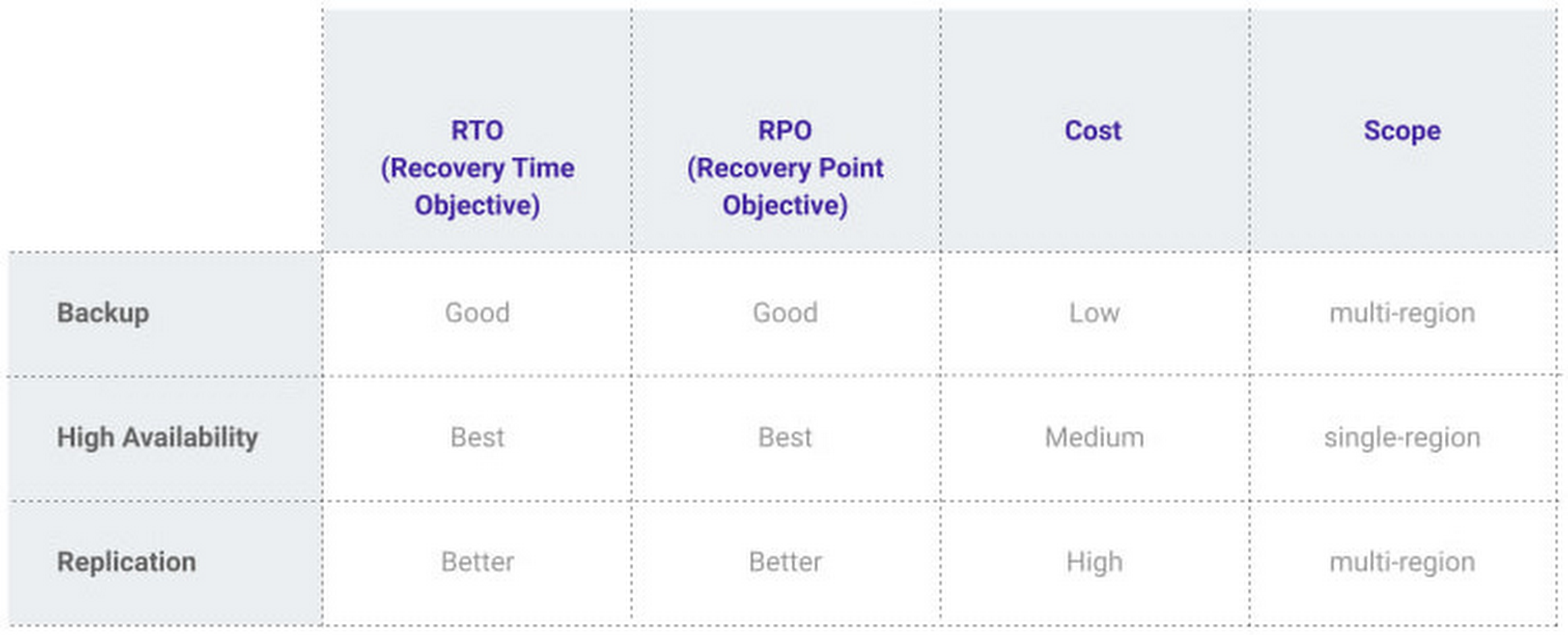
At Google, our Cloud SQL managed database service offers three fault tolerance mechanisms —backup, high availability, and replication—and there are three major factors to consider for each of them:
- RTO (recovery time objective): When a failure happens, how much time can be lost before significant harm occurs?
- RPO (recovery point objective): When a failure happens, how much data can be lost before significant harm occurs?
- Cost: How cost-effective is this solution?
We’ve heard from customers like Major League Baseball, HSBC, and Equifax that they have strict data-protection needs and require highly fault-tolerant multi-region applications—and they’ve all chosen Cloud SQL to meet those needs.
Let’s take a closer look at how the decision-making process plays out for each recovery solution.
High availability (HA)
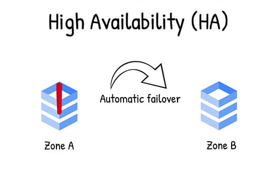
If your application is business critical, you require minimum RTO and zero RPO— a high availability configuration ensures that you and your customers are protected. If the primary instance fails, there’s another standby instance ready to take over with no data loss. There’s an additional cost here, but doing this manually brings a great operational cost, since you have to detect and verify the fault, do the failover, and make sure it’s correct—you can’t have two primary instances or you risk data corruption—then finally connect the application to the new database.
Cloud SQL removes all that complexity. Choose high availability for a given instance and we’ll replicate the data across multiple zones, synchronously, to each zone’s persistent disk. If an HA instance has a failure, you don’t have to think about when to fail over because Cloud SQL detects the failure and automatically initiates failover, for a full recovery and no data loss within minutes. Cloud SQL also moves the IP address during failover so your application can easily reconnect. MLB, for example, uses Cloud SQL high availability to serve prediction data to live games with minimal downtime. Dev/test instances don’t need those same guarantees, but can use local backups to recover from any potential failure.
Cross-region replica
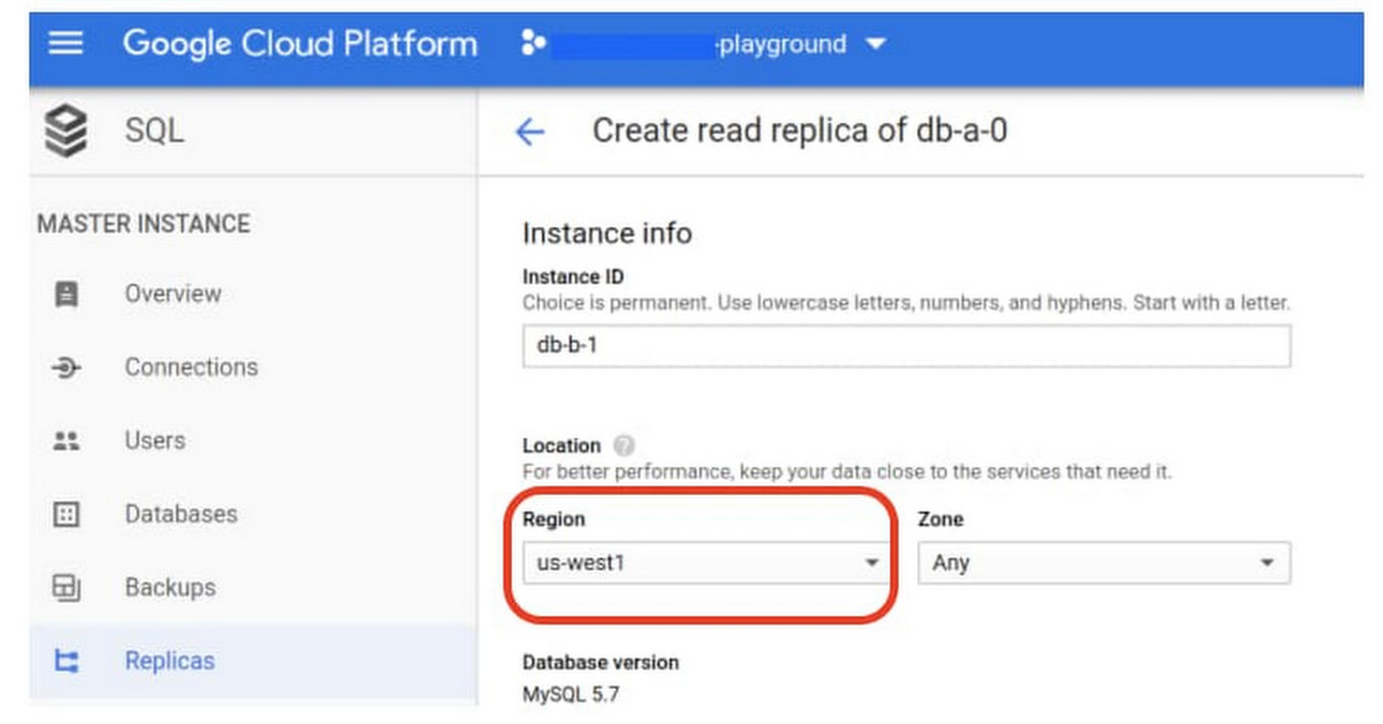
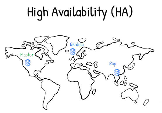
If a whole Google Cloud region goes down you still need your business to continue to run. That’s where cross-region replication comes in, a hot standby replica in another Google Cloud region provides RTO of minutes and RPO typically less than a minute . If you create a read replica in a region separate from your primary instance and you get hit with a regional outage, your application and database can start serving customers from another region within minutes. But this solution can be complex and enabling it yourself can be difficult and time-consuming. Securing cross-geography traffic demands end-to-end encryption and can bring connectivity issues too.
This is where the fully managed Cloud SQL solution shines. We offer MySQL, PostgreSQL and SQL Server database engines as a cross-region replication solution that’s easily configured and bolstered by Google’s interconnected global network. Just say, “I’m in U.S. East, I want to create a replica in U.S. West,” and it’s done, reliably and securely.
Backup
When you suffer data loss because of an operations error (for example, a bug in a script dropped your tables) or human error (for example, someone dropped the wrong table by accident), backups help you restore lost data to your Cloud SQL instance. Our low cost backup mechanism features point-in-time, granular recovery, meaning that if you accidentally delete data or something else goes wrong, you can ask for recovery of, for example, the state of that database down to the millisecond, such as Monday at 12:53pm. Your valuable data is replicated multiple times in multiple geographic locations automatically. This enables the automatic handling of failover in cases of major failure. You can always rest assured that your database is available and data is secure, even in the times of major failure crises.
Cloud SQL provides automated and on-demand backups. With automated backups, Google manages the backups so that you can easily restore them when required. Also, the scheduled backing is automatically taken by default. With on-demand backup, you can create a backup at any time. This could be useful if you are about to perform a risky operation on your database, as Cloud SQL lets you select a custom location for your backup data. When the backup is stored in multiple regions, and there’s an outage in the region that contains the source instance, you can restore a backup to a new or existing instance in a different region. This is also useful if your organization needs to comply with data residency regulations that require you to keep your backups within a specific geographic boundary.
Putting it all together
For critical workloads, MLB configures their Cloud SQL instances with backups, high availability, and cross-region replication. Doing so ensures they can recover from many failure types.
- To recover from human error (“Oops, I didn’t mean to delete that”), MLB uses backups and point-in-time recovery to recovery to a millisecond or specific database transaction
- To automatically recover from primary instance failures and zonal outages, MLB uses Cloud SQL’s high availability configuration
- To protect against regional outages, MLB uses cross-region replication
Creating a robust configuration, like MLB did, takes just a few minutes. Get started in our Console or review documentation.
Autoclass: Simplify and Automate Cost Optimization for Cloud Storage

3230
Of your peers have already read this article.
3:00 Minutes
The most insightful time you'll spend today!
There is a data explosion challenge that most IT admins and companies are tackling regularly. The cost-effectiveness, durability and scalability make object storage the first choice for unstructured data. Cloud Storage is an object storage service capable of storing data at exabyte scale and easily managing billions, if not trillions, of objects. However, cost optimization for data stored in object storage is a hard problem.
Choosing the right storage class for your data requires you to know about the access patterns for this data. However, if the access patterns are unknown or unpredictable, it’s often difficult for customers to choose the right storage class for their data. Data placement can have a significant impact on cost as the storage price for the archive class is 6% the storage price for the standard storage class. Having frequently accessed data in colder storage classes can lead to unexpected operations charges. Having data that is never accessed in standard storage can lead to large at-rest storage bills.
As IT administrators and organizations enable different applications and workloads to start leveraging object storage at massive scale, optimizing for cost is only getting exponentially harder to solve. As they migrate workloads to cloud they would like to have predictability and control in their overall storage spend. Wouldn’t it be great if there was a way to automatically place your data in the best storage class?
Introducing Autoclass – a new managed data placement service for Cloud Storage.
Simplifying Lifecycle Management while Reducing TCO
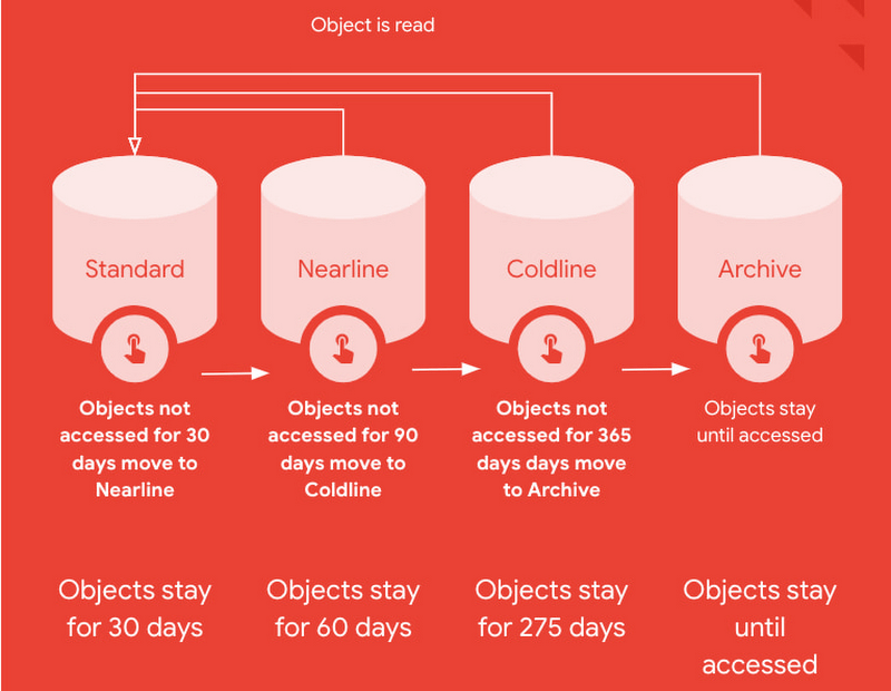
Autoclass is an easy to use bucket-level setting that simplifies and automates lifecycle management of all your Cloud Storage data based on last access time.
This is very useful for workloads with unpredictable and unknown access patterns. It automatically moves data that is not accessed to colder storage classes to reduce at-rest storage cost. When cold data is accessed, it is automatically promoted to Standard storage class to optimize the operations costs for future accesses.
Autoclass automatically delivers cost savings and removes inefficiencies by moving data to the storage class with the most favorable pricing for customer workloads.
It helps organizations achieve price predictability by removing surcharges associated with colder storage classes – there are no early deletion fees, retrieval fees or operations charges for class transitions when Autoclass is enabled on a bucket.
What are customers saying about Autoclass?
“Redivis is a data platform for academic research. We connect data managers with researchers to discover, understand, and analyze Petabytes of data. With Cloud Storage Autoclass, this shifts the paradigm in the research community,” said Ian Matthews, co-founder and CEO of Redivis Inc. “We can now keep more data for longer periods of time while reducing our costs. In fact, I’d estimate 90% of our data will benefit from Autoclass.”
Ian adds “Not only would it cost valuable engineering resources to build cost-optimization ourselves, but it would open us up to potentially costly mistakes in which we incur retrieval charges for prematurely archived data. Autoclass helps us reduce storage costs and achieve price predictability in a simple and automated way.”
Using Autoclass
With this release, Autoclass can be enabled when you create a new Cloud Storage bucket by using CLI, API, or Cloud Console. Once enabled on a bucket, Autoclass will manage the lifecycle of all objects that are uploaded to the bucket until disabled.
If you choose to disable Autoclass, all the objects in the bucket will remain in their current storage class. This disablement doesn’t require any data movement or any changes to storage classes of objects and hence, incurs no charge.
The support for enabling Autoclass on existing Cloud Storage buckets will be available in an upcoming release in 2023.
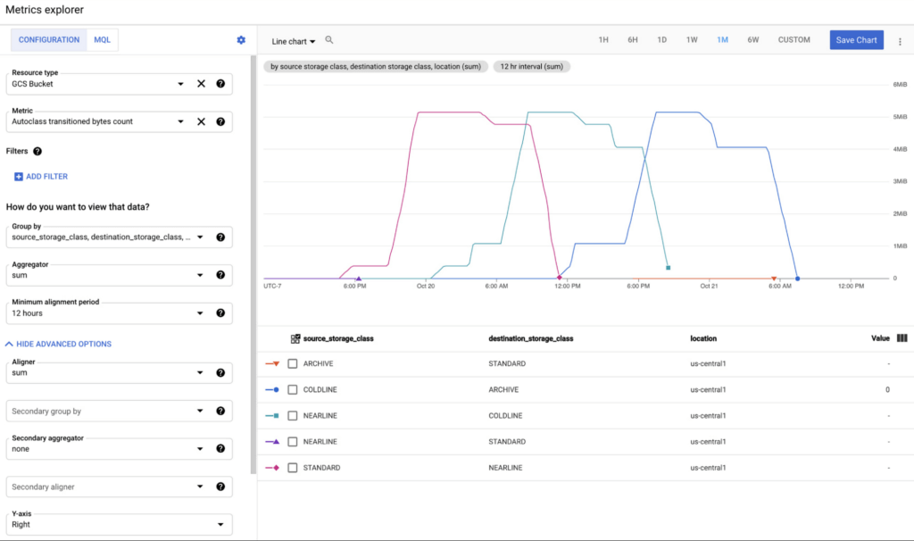
All transitions carried out by Autoclass can be observed using Cloud Monitoring dashboards. This provides easy observability and allows you to validate what Autoclass is doing for your data in an automated way. These dashboards can leverage 2 new Cloud metrics published for Autoclass:
- Number of objects transitioned by Autoclass (autoclass/transition_operation_count)
- Number of bytes transitioned between classes by Autoclass (autoclass/transitioned_bytes_count)
Getting Started
All Cloud Storage customers can enable Autoclass on their new buckets and realize the cost savings for themselves. For more information and detailed instructions on how to enable Autoclass, refer to the documentation here.
BigQuery Explainable AI for Demystifying the Inner Workings of ML Models. Now GA!

6570
Of your peers have already read this article.
2:00 Minutes
The most insightful time you'll spend today!
Explainable AI (XAI) helps you understand and interpret how your machine learning models make decisions. We’re excited to announce that BigQuery Explainable AI is now generally available (GA). BigQuery is the data warehouse that supports explainable AI in a most comprehensive way w.r.t both XAI methodology and model types. It does this at BigQuery scale, enabling millions of explanations within seconds with a single SQL query.
Why is Explainable AI so important? To demystify the inner workings of machine learning models, Explainable AI is quickly becoming an essential and growing need for businesses as they continue to invest in AI and ML. With 76% of enterprises now prioritizing artificial intelligence (AI) and machine learning (ML) over other initiatives in 2021 IT budgets, the majority of CEOs (82%) believe that AI-based decisions must be explainable to be trusted according to a PwC survey.
While the focus of this blogpost is on BigQuery Explainable AI, Google Cloud provides a variety of tools and frameworks to help you interpret models outside of BigQuery, such as with Vertex Explainable AI, which includes AutoML Tables, AutoML Vision, and custom-trained models.
So how does Explainable AI in BigQuery work exactly? And how might you use it in practice?
Two types of Explainable AI: global and local explainability
When it comes to Explainable AI, the first thing to note is that there are two main types of explainability as they relate to the features used to train the ML model: global explainability and local explainability.
Imagine that you have a ML model that predicts housing price (as a dollar amount), based on three features: (1) number of bedrooms, (2) distance to the nearest city center, and (3) construction date.
Global explainability (a.k.a. global feature importance) describes the features’ overall influence on the model and helps you understand if a feature had a greater influence than other features over the model’s predictions. For example, global explainability can reveal that the number of bedrooms and distance to city center typically has a much stronger influence than the construction date on predicting housing prices. Global explainability is especially useful if you have hundreds or thousands of features and you want to determine which features are the most important contributors to your model. You may also consider using global explainability as a way to identify and prune less important features to improve the generalizability of their models.
Local explainability (a.k.a. feature attributions) describes the breakdown of how each feature contributes towards a specific prediction. For example, if the model predicts that house ID#1001 has a predicted price of $230,000, local explainability would describe a baseline amount (e.g. $50,000) and how each of the features contributes on top of the baseline towards the predicted price. For example, the model may say that on top of the baseline of $50,000, having 3 bedrooms contributed an additional $50,000, close proximity to the city center added $100,000, and construction date of 2010 added $30,000, for a total predicted price of $230,000. In essence, understanding the exact contribution of each feature used by the model to make each prediction is the main purpose of local explainability.
What ML models does BigQuery Explainable AI apply to?
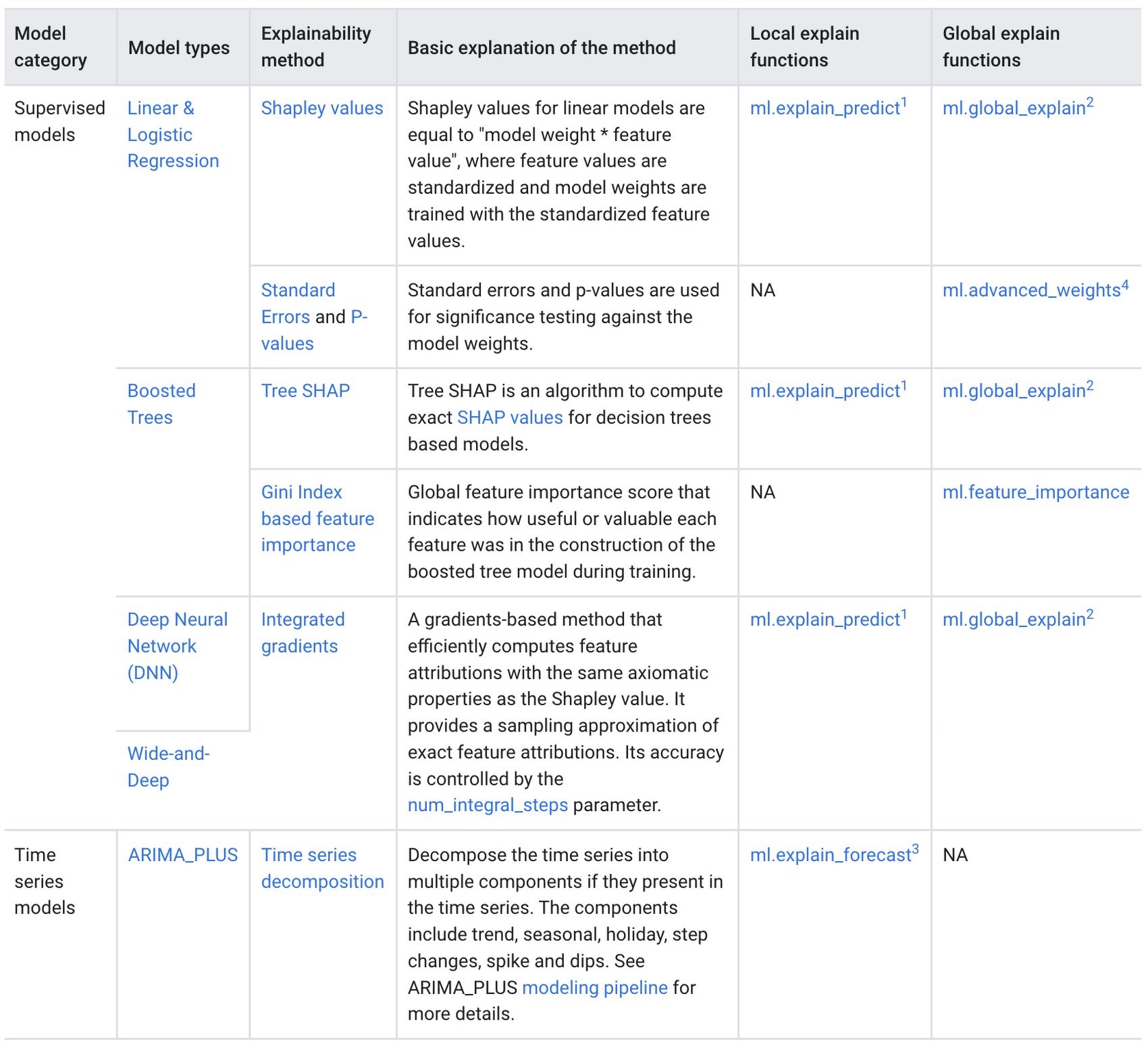
BigQuery Explainable AI applies to a variety of models, including supervised learning models for IID data and time series models. The documentation for BigQuery Explainable AI provides an overview of the different ways of applying explainability per model. Note that each explainability method has its own way of calculation (e.g. Shapley values), which are covered more in-depth in the documentation.
Examples with BigQuery Explainable AI
In this next section, we will show three examples of how to use BigQuery Explainable AI in different ML applications:
Regression models with BigQuery Explainable AI
Let’s use a boosted tree regression model to predict how much a taxi cab driver will receive in tips for a taxi ride, based on features such as number of passengers, payment type, total payment and trip distance. Then let’s use BigQuery Explainable AI to help us understand how the model made the predictions in terms of global explainability (which features were most important?) and local explainability (how did the model arrive at each prediction?).
The taxi trips dataset comes from the BigQuery public datasets and is publicly available in the table: bigquery-public-data.new_york_taxi_trips.tlc_yellow_trips_2018.
First, you can train a boosted tree regression model.
CREATE OR REPLACE MODEL bqml_tutorial.taxi_tip_regression_modelOPTIONS (model_type='boosted_tree_regressor',input_label_cols=['tip_amount'],max_iterations = 50,tree_method = 'HIST',subsample = 0.85,enable_global_explain = TRUE) ASSELECTvendor_id,passenger_count,trip_distance,rate_code,payment_type,total_amount,tip_amountFROM`bigquery-public-data.new_york_taxi_trips.tlc_yellow_trips_2018`WHERE tip_amount >= 0LIMIT 1000000
Now let’s do a prediction using ML.PREDICT, which is the standard way in BigQuery ML to make predictions without explainability.
SELECT *FROMML.PREDICT(MODEL bqml_tutorial.taxi_tip_regression_model,(SELECT"0" AS vendor_id,1 AS passenger_count,CAST(5.85 AS NUMERIC) AS trip_distance,"0" AS rate_code,"0" AS payment_type,CAST(55.56 AS NUMERIC) AS total_amount))

But you might wonder—how did the model generate this prediction of ~11.077?
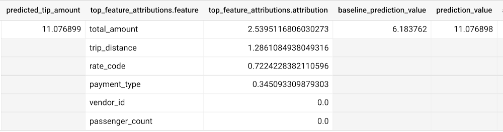
BigQuery Explainable AI can help us answer this question. Instead of using ML.PREDICT, you use ML.EXPLAIN_PREDICT with an additional optional parameter top_k_features. ML.EXPLAIN_PREDICT extends the capabilities of ML.PREDICT by outputting several additional columns that explain how each feature contributes to the predicted value. In fact, since ML.EXPLAIN_PREDICT includes all the output from ML.PREDICT anyway, you may want to consider using ML.EXPLAIN_PREDICT every time instead.
SELECT *FROMML.EXPLAIN_PREDICT(MODEL bqml_tutorial.taxi_tip_regression_model,(SELECT"0" AS vendor_id,1 AS passenger_count,CAST(5.85 AS NUMERIC) AS trip_distance,"0" AS rate_code,"0" AS payment_type,CAST(55.56 AS NUMERIC) AS total_amount),STRUCT(6 AS top_k_features))
The way to interpret these columns is:
Σfeature_attributions + baseline_prediction_value = prediction_value
Let’s break this down. The prediction_value is ~11.077, which is simply the predicted_tip_amount. The baseline_prediction_value is ~6.184, which is the tip amount for an average instance. top_feature_attributions indicates how much each of the features contributes towards the prediction value. For example, total_amount contributes ~2.540 to the predicted_tip_amount.
ML.EXPLAIN_PREDICT provides local feature explainability for regression models. For global feature importance, see the documentation for ML.GLOBAL_EXPLAIN.
Classification models with BigQuery Explainable AI
Let’s use a logistic regression model to show you an example of BigQuery Explainable AI with classification models. We can use the same public dataset as before: bigquery-public-data.new_york_taxi_trips.tlc_yellow_trips_2018.
Train a logistic regression model to predict the bracket of the percentage of the tip amount out of the taxi bill.
CREATE OR REPLACE MODEL bqml_tutorial.taxi_tip_classification_modelOPTIONS(model_type='logistic_reg',input_label_cols=['tip_bucket'],enable_global_explain=true) ASSELECTvendor_id,passenger_count,trip_distance,rate_code,payment_type,total_amount,CASEWHEN tip_amount > total_amount*0.20 THEN '20% or more'WHEN tip_amount > total_amount*0.15 THEN '15% to 20%'WHEN tip_amount > total_amount*0.10 THEN '10% to 15%'ELSE '10% or less'END AS tip_bucketFROM`bigquery-public-data.new_york_taxi_trips.tlc_yellow_trips_2018`WHERE tip_amount >= 0LIMIT 1000000
Next, you can run ML.EXPLAIN_PREDICT to get both the classification results and the additional information for local feature explainability. For global explainability, you can use ML.GLOBAL_EXPLAIN. Again, since ML.EXPLAIN_PREDICT includes all the output from ML.PREDICT anyway, you may want to consider using ML.EXPLAIN_PREDICT every time instead.
SELECT *FROMML.EXPLAIN_PREDICT(MODEL bqml_tutorial.taxi_tip_classification_model,(SELECT"0" AS vendor_id,1 AS passenger_count,CAST(5.85 AS NUMERIC) AS trip_distance,"0" AS rate_code,"0" AS payment_type,CAST(55.56 AS NUMERIC) AS total_amount),STRUCT(6 AS top_k_features))
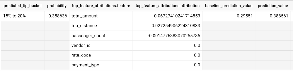
Similar to the regression example earlier, the formula is used to derive the prediction_value:
Σfeature_attributions + baseline_prediction_value = prediction_value
As you can see in the screenshot above, the baseline_prediction_value is ~0.296. total_amount is the most important feature in making this specific prediction, contributing ~0.067 to the prediction_value, though followed by trip_distance. The feature passenger_count contributes negatively to prediction_value by -0.0015. The features vendor_id, rate_code, and payment_type did not seem to contribute much to the prediction_value.
You may wonder why the prediction_value of ~0.389 doesn’t equal the probability value of ~0.359. The reason is that unlike for regression models, for classification models, prediction_value is not a probability score. Instead, prediction_value is the logit value (i.e., log-odds) for the predicted class, which you could separately convert to probabilities by applying the softmax transformation to the logit values. For example, a three-class classification has a log-odds output of [2.446, -2.021, -2.190]. After applying the softmax transformation, the probability of these class predictions is [0.9905, 0.0056, 0.0038].
Time-series forecasting models with BigQuery Explainable AI
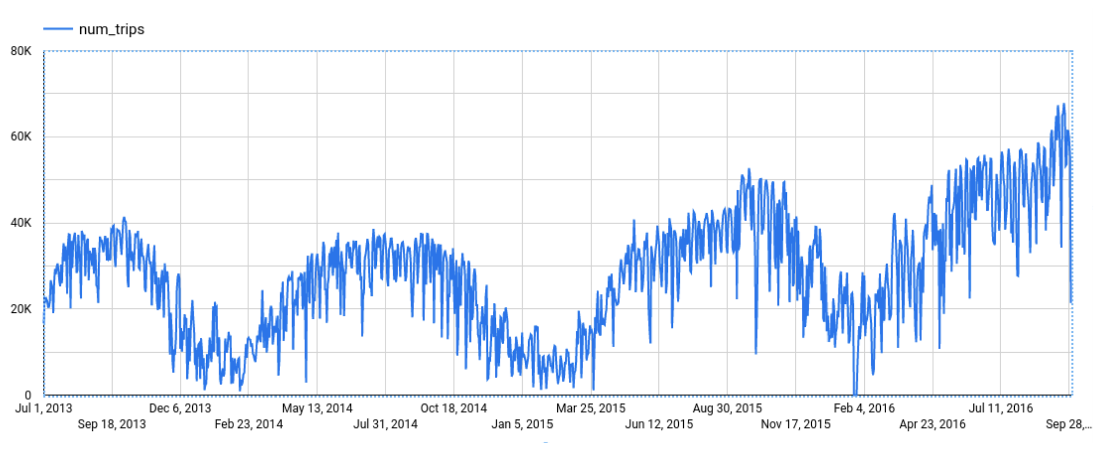
Explainable AI for forecasting provides more interpretability into how the forecasting model came to its predictions. Let’s go through an example of forecasting the number of bike trips in NYC using the new_york.citibike_trips public data in BigQuery.
You can train a time-series model ARIMA_PLUS:
CREATE OR REPLACE MODEL bqml_tutorial.nyc_citibike_arima_modelOPTIONS(model_type = 'ARIMA_PLUS',time_series_timestamp_col = 'date',time_series_data_col = 'num_trips',holiday_region = 'US') ASSELECTEXTRACT(DATE from starttime) AS date,COUNT(*) AS num_tripsFROM`bigquery-public-data.new_york.citibike_trips`GROUP BY dateNext, you can first try forecasting without explainability using ML.FORECAST:SELECT*FROMML.FORECAST(MODEL bqml_tutorial.nyc_citibike_arima_model,STRUCT(365 AS horizon, 0.9 AS confidence_level))
This function outputs the forecasted values and the prediction interval. Plotting it in addition to the input time series gives the following figure.
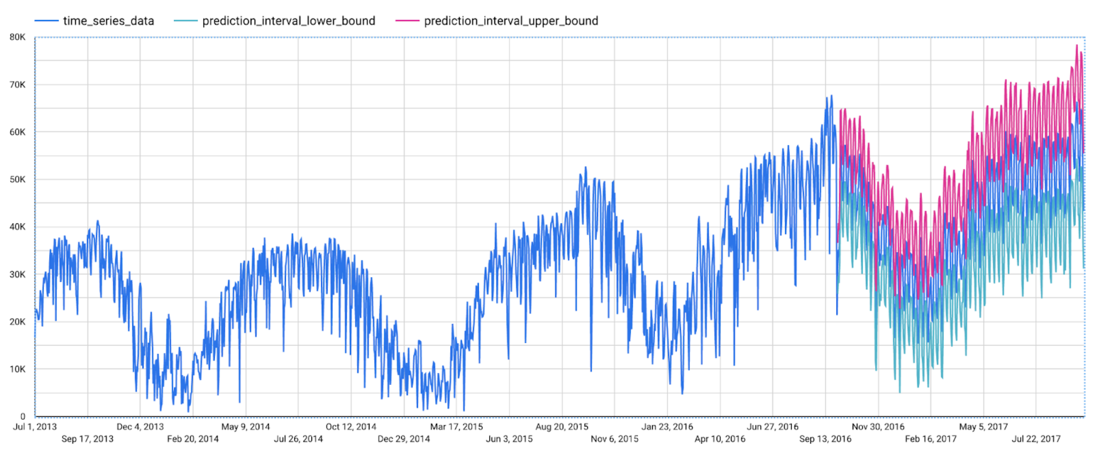
But how does the forecasting model arrive at its predictions? Explainability is especially important if the model ever generates unexpected results.
With ML.EXPLAIN_FORECAST, BigQuery Explainable AI provides extra transparency into the seasonality, trend, holiday effects, level (step) changes, and spikes and dips outlier removal. In fact, since ML.EXPLAIN_FORECAST includes all the output from ML.FORECAST anyway, you may want to consider using ML.EXPLAIN_FORECAST every time instead.
SELECT*FROMML.EXPLAIN_FORECAST(MODEL bqml_tutorial.nyc_citibike_arima_model,STRUCT(365 AS horizon, 0.9 AS confidence_level))
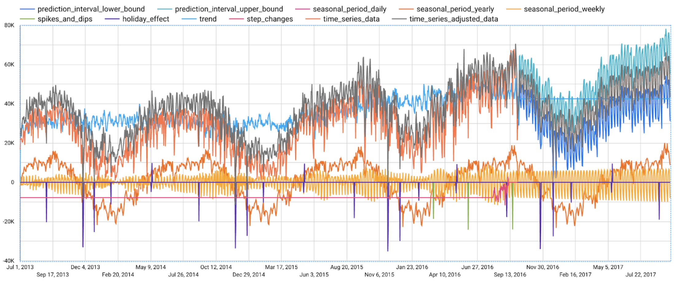
Compared to the previous figure which only shows the forecasting results, this figure shows much richer information to explain how the forecast is made.
First, it shows how the input time series is adjusted by removing the spikes and dips anomalies, and by compensating the level changes. That is:
time_series_adjusted_data = time_series_data - spikes_and_dips - step_changes
Second, it shows how the adjusted input time series is decomposed into different components such as both weekly and yearly seasonal components, holiday effect component and trend component. That is
time_series_adjusted_data = trend + seasonal_period_yearly + seasonal_period_weekly + holiday_effect + residual
Finally, it shows how these components are forecasted separately to compose the final forecasting results. That is:
time_series_data = trend + seasonal_period_yearly + seasonal_period_weekly + holiday_effect
For more information on these time series components, please see the documentation here.
Conclusion
With the GA of BigQuery Explainable AI, we hope you will now be able to interpret your machine learning models with ease.
Thanks to the BigQuery ML team, especially Lisa Yin, Jiashang Liu, Amir Hormati, Mingge Deng, Jerry Ye and Abhinav Khushraj. Also thanks to the Vertex Explainable AI team, especially David Pitman and Besim Avci.
6188
Of your peers have already watched this video.
16:00 Minutes
The most insightful time you'll spend today!
Easy Access to Stream Analytics with Google Cloud
By 2025, more than a quarter of the data created in the global datasphere will be real-time in nature.
“This is important because in the real-time world, “the window of opportunity diminishes and goes away really fast. You want to be able to respond to your customer needs, their asks, and be able to do prediction or maybe detect some problem and really respond to it really fast,” says Evren Eryurek, Director of Product Management for Stream Analytics at Google Cloud.
Today, streaming analysis of application and user events only continue to become more central to how every business operates. With this development comes an accompanying rise in customer expectations for businesses to be aware, prepared, and delivering real-time solutions. Is your business ready?
In this session, Eryurek will showcase Google Cloud’s latest developments to enable easy access to creation and management of real-time data driven experiences.
Learn the latest about the products powering Google’s streaming capabilities and hear directly from the team bringing them to life.
More Relevant Stories for Your Company

What is Google Cloud SQL?
Cloud SQL is a fully managed relational database for MySQL, PostgreSQL, and SQL Server. It reduces maintenance cost and automates database provisioning, storage capacity management, replication, and backups. It offers quick setup, with standard connection drivers and built-in migration tools. How Do You Set It Up? Cloud SQL is easy

Carbon Health: Transforming outcomes with Connected Sheets for Looker
Everyone wants affordable, quality healthcare but not everyone has it. A 2021 report by the Commonwealth Fund ranked the U.S. in last place among 11 high-income countries in healthcare access.1 Carbon Health is working to change that. We are doing so by combining the best of virtual care, in-person visits,
Recommendations for Modelling SAP Data inside BigQuery
Over the past few years, many organizations have experienced the benefits of migrating their SAP solutions to Google Cloud. But this migration can do more than reduce IT maintenance costs and make data more secure. By leveraging BigQuery, SAP customers can complement their SAP investments and gain fresh insights by consolidating enterprise

Experts’ Guideline for Personalizing Platforms with the Right Recommendation System on Google Cloud
Over the past two decades, consumers have become accustomed to receiving personalized recommendations in all facets of their online life. Whether that be recommended products while shopping on Amazon, a curated list of apps in the Google Play store, or relevant videos to watch next on YouTube. In fact, in
