





Recommendations for Modelling SAP Data inside BigQuery
8395
Of your peers have already read this article.
4:00 Minutes
The most insightful time you'll spend today!
Over the past few years, many organizations have experienced the benefits of migrating their SAP solutions to Google Cloud. But this migration can do more than reduce IT maintenance costs and make data more secure. By leveraging BigQuery, SAP customers can complement their SAP investments and gain fresh insights by consolidating enterprise data and easily extending it with powerful datasets and machine learning from Google.
BigQuery is a leading cloud data warehouse, fully managed and serverless, and allows for massive scale, supporting petabyte-scale queries at super-fast speeds. It can easily combine SAP data with additional data sources, such as Google Analytics or Salesforce, and its built-in machine learning lets users operationalize machine learning models using standard SQL — all at a comparatively low cost.
If your SAP-powered organization is looking to supercharge its analytics with the strength of BigQuery, read on for considerations and recommendations for modeling with SAP data. These guidelines are based on our real-world implementation experience with customers and can serve as a roadmap to the analytics capabilities your business needs.
Considerations for data replication
Like most technology journeys, this one should start with a business objective. Keeping your intended business value and goals in mind is critical to making the right decisions in the early steps of the design process.
When it comes to replicating the data from an SAP system into BigQuery, there are multiple ways to do it successfully. Decide which method will work best for your organization by answering these questions:
- Does your business need real-time data? Will you need to time travel into past data?
- Which external datasets will you need to join with the replicated data?
- Are the source structures or business logic likely to change? Will you be migrating the SAP source systems any time soon? For instance, will you be moving from SAP ECC to SAP S/4HANA?
You’ll also need to determine whether replication should be done on a table-by-table basis or whether your team can source from pre-built logic. This decision, along with other considerations such as licensing, will influence which replication tool you should use.
Replicating on a table-by-table basis
Replicating tables, especially standard tables in their raw form, allows sources to be reused and ensures more stability of the source structure and functional output. For example, the SAP table for sales order headers (VBAK) is very unlikely to change its structure across different versions of SAP, and the logic that writes to it is also unlikely to change in a way that affects a replicated table.
Something else to consider: Reconciliation between the source system and the landing table in BigQuery is linear when comparing raw tables, which helps avoid issues in consolidation exercises during critical business processes, such as period-end closing. Since replicated tables aren’t aggregated or subject to process-specific data transformation, the same replicated columns can be reused in different BigQuery views. You can, for instance, replicate the MARA table (the material master) once and use it in as many models as needed.
Replicating pre-built logic
If you replicate pre-built models, such as those from SAP extractors or CDS views, you don’t need to build the logic in BigQuery, since you’re using existing logic. Some of these extraction objects have embedded delta mechanisms, which may complement a replication tool that can’t handle deltas. This will save initial development time, but it can also lead to challenges if you create new columns, or if customizations or upgrades change the logic behind the extraction.
It’s also important to note that different extraction processes may transform and load the same source columns multiple times, which creates redundancy in BigQuery and can lead to higher maintenance needs and costs. However, replicating pre-built models may still be a good choice, since doing so can be especially useful for logic that tends to be immutable, such as flattening a hierarchy, or logic that is highly complex.
How you approach replication will also depend on your long-term plans and other key factors — for example, the availability (and curiosity) of your developers, and the time or effort they can put into applying their SQL knowledge to a new data warehouse.
With either replication approach, bear in mind when designing your replication process that BigQuery is meant to be an append-always database — so post-processing of data and changes will be required in both cases.
Processing data changes
The replication tool you choose will also determine how data changes are captured (known as CDC – change data capture). If the replication tool allows for it (for example as SAP SLT does) the same patterns described in the CDC with BigQuery documentation also apply to SAP data.
Because some data, like transactions, are known to be less static than others (e.g., master data), you need to decide what should be scanned in real time, what will require immediate consistency, and what can be processed in batches to manage costs. This decision will be based on the reporting needs from the business.
Consider the SAP table BUT000, containing our example master data for business partners, where we have replicated changes from an SAP ERP system:
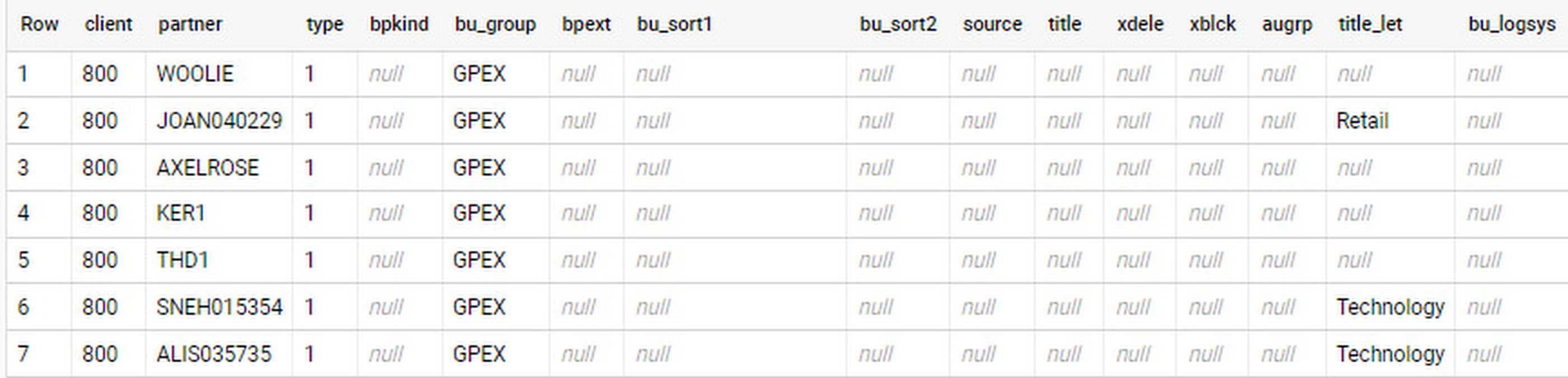
In an append-always replication in BigQuery, all updates are received as new records. For example, deleting a record in the source will be represented as a new record in BigQuery with a deletion flag. This applies to whether the records are coming from raw tables like BUT000 itself or pre-aggregated data, as from a BW extractor or a CDS view.
Let’s take a closer look at data coming particularly from the partners “LUCIA” and “RIZ”. The operation flag tells us whether the new record in BigQuery is an insert (I), update (U) or deletion (D), while the timestamps help us identify the latest version of our business partner.
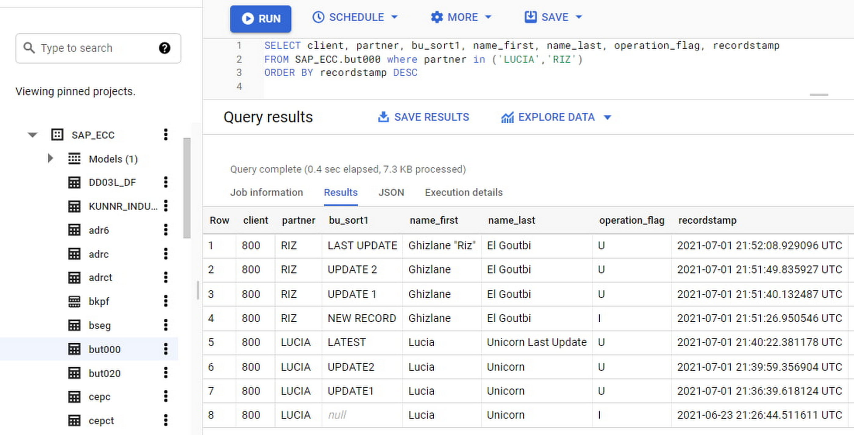
If we want to find the latest updated record for the partners LUCIA and RIZ, this is what the query would look like:
SELECT partner,ARRAY_AGG(i1 ORDER BY i1.recordstamp DESC LIMIT 1) AS rowFROM SAP_ECC.but000 i1WHERE partner in ('LUCIA','RIZ')GROUP BY partner
With the following result:
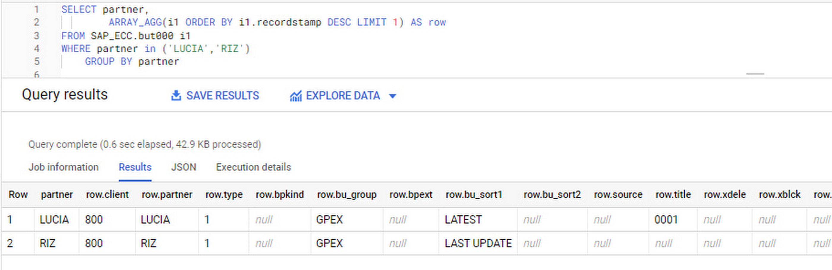
After identifying stale records for “LUCIA” and “RIZ” business partners, we can proceed to deleting all stale records for “LUCIA” if we do not want to retain the history. In this example, we are using a different table to which the same replication has been done, for the purpose of comparison and to check that all stale records have been deleted for the selection made and that we only kept last updated records. For example:
DELETE SAP_HANA.but000 i1WHEREi1.recordstamp < TIMESTAMP_SUB(CURRENT_TIMESTAMP(), INTERVAL 3 HOUR) ANDi1.recordstamp < (SELECT MAX(recordstamp) FROM SAP_HANA.but000 i2WHEREi1.partner = i2.partnerand partner="LUCIA")
You can also use the following query to retrieve stale records for “LUCIA” partner before moving forward with deletion
SELECT partner, operation_flag, recordstamp FROM SAP_HANA.but000 i1WHEREi1.recordstamp < TIMESTAMP_SUB(CURRENT_TIMESTAMP(), INTERVAL 3 HOUR)ANDi1.recordstamp < (SELECT MAX(recordstamp) FROM SAP_HANA.but000 i2WHEREi1.partner = i2.partnerand partner="LUCIA")
Which produces all of the records, except the latest update:

Partitioning and clustering
To limit the number of records scanned in a query, save on cost and achieve the best performance possible, you’ll need to take two important steps: determine partitions and create clusters.
Partitioning
A partitioned table is one that’s divided into segments, called partitions, which make it easier to manage and query your data. Dividing a large table into smaller partitions improves query performance and controls costs because it reduces the number of bytes read by a query.
You can partition BigQuery tables by:
- Time-unit column: Tables are partitioned based on a “timestamp,” “date,” or “datetime” column in the table.
- Ingestion time: Tables are partitioned based on the timestamp recorded when BigQuery ingested the data.
- Integer range: Tables are partitioned based on an integer column.
Partitions are enabled when the table is created, as in the example below. A great tip is to always include the partition filter as shown on the left-hand side of the query.

Clustering
Clustering can be created on top of partitioned tables by applying the fields that are likely to be used for filtering. When you create a clustered table in BigQuery, the table data is automatically organized based on the contents of one or more of the columns in the table’s schema. The columns you specify are then used to colocate related data.
Clustering can improve the performance of certain query types — for example, queries that use filter clauses or that aggregate data. It makes a lot of sense to use them for large tables such as ACDOCA, the table for accounting documents in SAP S/4HANA. In this case, the timestamp could be used for partitioning, and common filtering fields such as the ledger, company code, and fiscal year could be used to define the clusters.
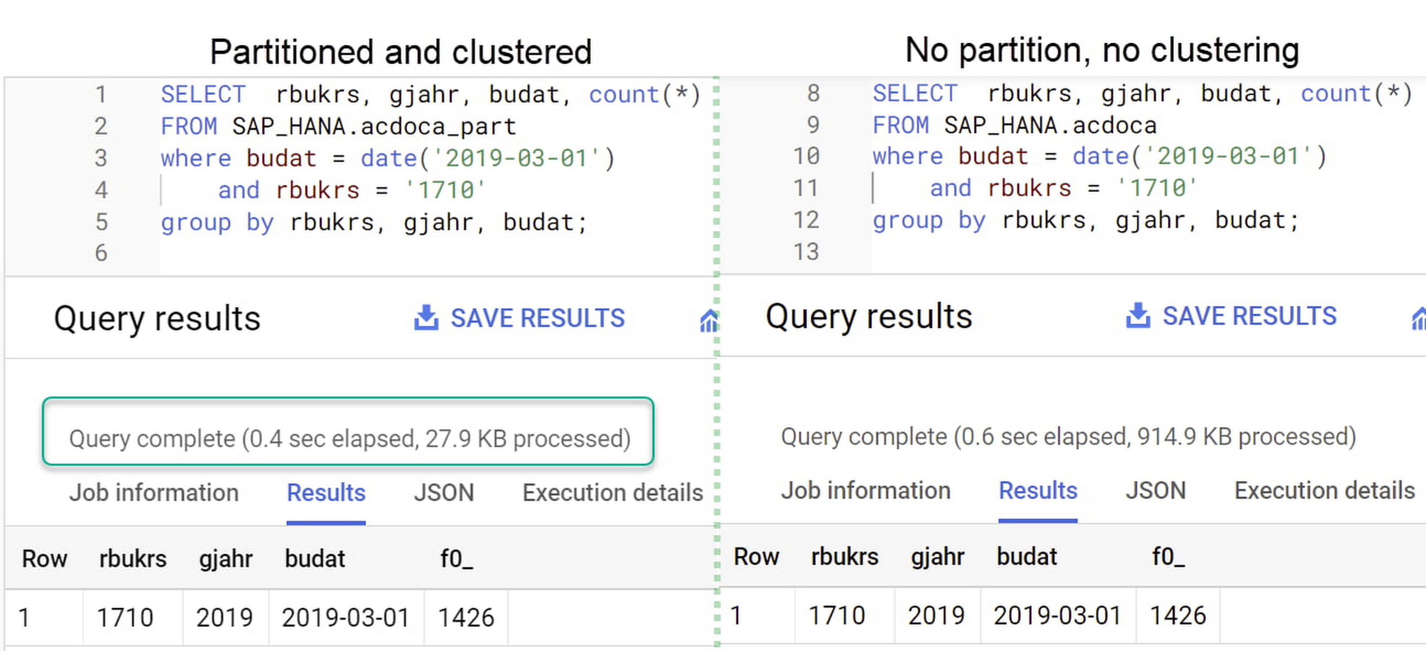
A great feature is that BigQuery will also periodically recluster the data automatically.
Materialized views
In BigQuery, materialized views are precomputed views that periodically cache the results of a query for better performance and efficiency. BigQuery uses precomputed results from materialized views and, whenever possible, reads only the delta changes from the base table to compute up-to-date results quickly. Materialized views can be queried directly or can be used by the BigQuery optimizer to process queries to the base table.
Queries that use materialized views are generally completed faster and consume fewer resources than queries that retrieve the same data only from the base table. If workload performance is an issue, materialized views can significantly improve the performance of workloads that have common and repeated queries. While materialized views currently only support single tables, they are very useful common and frequent aggregations like stock levels or order fulfillment.
Further tips on performance optimization while creating select statements can be found in the documentation for optimizing query computation.
Deployment pipeline and security
For most of the work you’ll do in BigQuery, you’ll normally have at least two delivery pipelines running — one for the actual objects in BigQuery and the other to keep the data staging, transforming, and updated as intended within the change-data-capture flows. Note that you can use most existing tools for your Continuous Integration / Continuous Deployment (CI/CD) pipeline — one of the benefits of using an open system like BigQuery. But, if your organization is new to CI/CD pipelines, this is a great opportunity to gradually gain experience. A good place to start is to read our guide for setting up a CI/CD pipeline for your data-processing workflow.
When it comes to access and security, most end-users will only have access to the final version of the BigQuery views. While row and column-level security can be applied, as in the SAP source system, separation of concerns can be taken to the next level by splitting your data across different Google Cloud projects and BigQuery datasets. While it’s easy to replicate data and structures across your datasets, it’s a good idea to define the requirements and naming conventions early in the design process so you set it up properly from the start.
Start driving faster and more insightful analytics
The best piece of advice we can give you is this: Try it yourself. Anyone with SQL knowledge can get started using the free BigQuery tier. New customers get $300 in free credits to spend on Google Cloud during the first 90 days. All customers get 10 GB storage and up to 1 TB queries/month, completely free of charge. In addition to discovering the massive processing capabilities, embedded machine learning, multiple integration tools, and cost benefits, you’ll soon discover how BigQuery can simplify your analytics tasks.
If you need additional assistance, our Google Cloud Professional Services Organization (PSO) and Customer Engineers will be happy to help show you the best path forward for your organization. For anything else, contact us at cloud.google.com/contact.
The Query Execution Graph: Your Key to Better BigQuery Analytics

3070
Of your peers have already read this article.
2:30 Minutes
The most insightful time you'll spend today!
BigQuery offers strong query performance, but it is also a complex distributed system with many internal and external factors that can affect query speed. When your queries are running slower than expected or are slower than prior runs, understanding what happened can be a challenge.
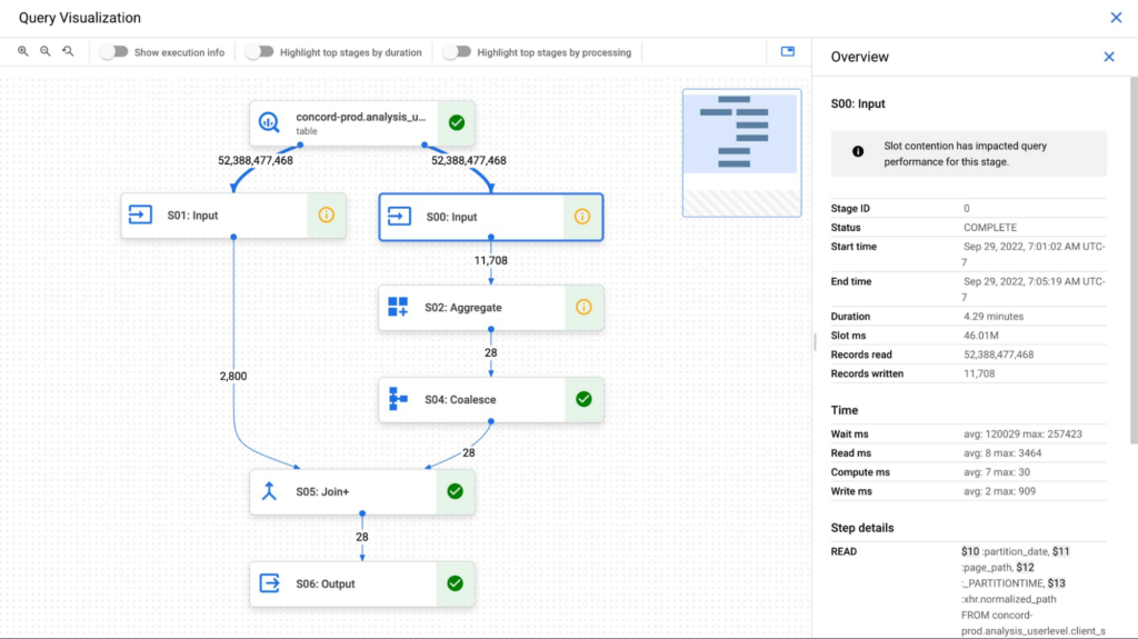
The query execution graph provides an intuitive interface for inspecting query execution details. By using it, you can review the query plan information in graphical format for any query, whether running or completed.
You can also use the query execution graph to get performance insights for queries. Performance insights provide best-effort suggestions to help you improve query performance. Since query performance is multi-faceted, performance insights might only provide a partial picture of the overall query performance.
Execution graph
When BigQuery executes a query job, it converts the declarative SQL statement into a graph of execution, broken up into a series of query stages, which themselves are composed of more granular sets of execution steps. The query execution graph provides a visual representation of the execution stages and shows the corresponding metrics. Not all stages are made equal. Some are more expensive and time consuming than others. The execution graph provides toggles for highlighting critical stages, which makes it easier to spot the potential performance bottlenecks in the query.
Query performance insights
In addition to the detailed execution graph BigQuery also provides specific insights on possible factors that might be slowing query performance.
Slot contention
When you run a query, BigQuery attempts to break up the work needed by your query into tasks. A task is a single slice of data that is input into and output from a stage. A single slot picks up a task and executes that slice of data for the stage. Ideally, BigQuery slots execute tasks in parallel to achieve high performance. Slot contention occurs when your query has many tasks ready for slots to start executing, but BigQuery can’t get enough available slots to execute them.
Insufficient shuffle quota
Before running your query, BigQuery breaks up your query’s logic into stages. BigQuery slots execute the tasks for each stage. When a slot completes the execution of a stage’s tasks, it stores the intermediate results in shuffle. Subsequent stages in your query read data from shuffle to continue your query’s execution. Insufficient shuffle quota occurs when you have more data that needs to get written to shuffle than you have shuffle capacity.
Data input scale change
Getting this performance insight indicates that your query is reading at least 50% more data for a given input table than the last time you ran the query and hence experiencing query slowness. You can use table change history to see if the size of any of the tables used in the query has recently increased.
What’s next?
We continue to work on improving the visualization of the graph. We are working on adding additional metrics to each step and adding more performance insights that will make query diagnosis significantly easier. We are just getting started.
Migrating MySQL to Spanner? Here’s What You Need to Know

5607
Of your peers have already read this article.
2:00 Minutes
The most insightful time you'll spend today!
Since its initial release in 1995, MySQL has not only been the de-facto database for many data storage needs, but has gathered much attention over the years as one of the most well-recognized databases around when it comes to Relational Database Management Systems and transactional data processing.
Any application in retail, e-commerce, or banking has likely had its fair share of business depending on a relational database for its transactional needs. Many of these applications are built on MySQL due to its flexibility, open source nature, and strong community support.
Whether in the context of a migration from a relational database (like MySQL or PostgreSQL) , migration from a NoSQL database (like Cassandra), or a green grass workload, many companies turn to Cloud Spanner seeking a high availability SLA (99.99% for regional instances and 99.999% for multi region instances), unlimited scale, and low operational overhead – no patching required, no maintenance or other planned downtimes, just to name a few benefits.
The tooling and open source ecosystem around Spanner has evolved and grown ever since the service was introduced. HarbourBridge is a part of this ecosystem, and it’s meant to help customers port their existing MySQL or PostgreSQL schema to a Cloud Spanner schema.
Application Migration Tips
Despite helpful tools like HarbourBridge, database migrations are never trivial. Here are a few things to pay attention to when migrating from MySQL to Spanner, and how to update your application logic to address them.
Note – The following snippets use the PHP client for Cloud Spanner. A couple of the snippets reference a partial Magento port that our friends over at Searce have been working on. Once you understand the operations, you should be able to implement the same in any of the other languages that Cloud Spanner supports.
Cloud spanner enforces strict data types
In a MySQL query, the value of an attribute can be referenced as either a string or an integer. Example:
- select * from catalog_eav_attribute where attribute_id = 46;
- select * from catalog_eav_attribute where attribute_id = “46”;
Both are valid and equivalent.
In Cloud Spanner, the query will return an error if you try to reference an integer type by using a string representation.
Here is an example of a working query from Cloud Spanner:
- select * from catalog_eav_attribute where attribute_id = 46; — this will work
- Select * from catalog_eav_attribute where attribute_id = “46” — will fail, since we are supplying a string with “46”
You may use a function like the following to assist you with such transformations.
/*** Formats the SQL for Cloud Spanner* Example* Input SQL : <select statement> WHERE* (`product_id` = '340') ORDER BY position ASC* Output SQL : <select statement> WHERE* (`product_id` = 340) ORDER BY position ASC* In the above example integer*`340` is sanitized by removing single quotes.* Sanitization is required since Cloud Spanner* has strict typing* @param string $sql* @return string $sql*/public function sanitizeSql(string $sql){if (preg_match_all("/('[^']*')/", $sql, $m)) {$matches = array_shift($m);for($i = 0; $i < count($matches); $i++) {$curr = $matches[$i];$curr = filter_var($curr,FILTER_SANITIZE_NUMBER_INT);if (is_numeric($curr)) {$sql = str_replace($matches[$i],$curr, $sql);}}}return $sql;}
Using sequences in primary keys is not a Spanner best practice
Cloud Spanner does not implement a sequence generator, and it is not a Spanner best practice to use sequential IDs because doing so can cause hotspotting.
An alternative mechanism of generating a unique primary key is to use a UUID or any other similar mechanisms that result in non-sequential values. For more information, please refer to this article.
In order to convert all existing primary keys to a UUID pattern, you can change the schema using the snippet here
You may use this code snippet to modify the application code to generate the UUID for the auto increment. There are other ways to do this as well, such as using PHP built-in uniqid function.
/*** Generate UUID.* @return string*/public function getAutoIncrement(){if (function_exists('com_create_guid') === true) {return trim(com_create_guid(), '{}');}return sprintf('%04X%04X-%04X-%04X-%04X-%04X%04X%04X',mt_rand(0, 65535), mt_rand(0, 65535),mt_rand(0, 65535), mt_rand(16384, 20479),mt_rand(32768, 49151), mt_rand(0, 65535),mt_rand(0, 65535), mt_rand(0, 65535));}
Implicit casting and the need for explicit casting of field data types
Both MySQL and Cloud Spanner follow the SQL standard, hence much of the query syntax is the same. One notable difference is that the Cloud Spanner field types are implicitly cast to an appropriate data type out of the ones mentioned here. When implicit casting of the field type fails, Spanner returns a read error, so it would be safer to perform the casting to the appropriate type when issuing the SELECT statement.
Modify application code to cast to respective data type before execution of query.
$con = $this->getSpannerConnection();/*** Cloud Spanner follows strict type so cast the columns appropriately*/$select = $con->addCast($select, "`t_d`.`value`", 'string');$select = $con->addCast($select, "`t_s`.`value`", 'string');$select = $con->addCast($select, "IF(t_s.value_id IS NULL,t_d.value, t_s.value)", 'string');$values = $con->fetchAll($select);
Modify the application code to cast the column to its respective type
/*** Cast the column with type* @param string $sql* @param string $col* @param string $type* @return string*/public function addCast(string $sql,string $col, string $type){$cast = "cast(".$col." as ".$type.")";return str_replace($col, $cast, $sql);}
Using interleaved tables to improve read performance
Cloud Spanner’s table interleaving is a great choice for many parent-child relationships where the child table’s primary key includes the parent table’s primary key columns. Interleaving ensures that child rows are collocated with their parent rows, which can significantly improve query performance.
Refer to the statements here for a few samples of creating interleaved tables. To learn more about table interleaving, visit the documentation.
Conclusion
Database migrations are complicated. Hopefully, using HarbourBridge and the list of tips in this article can make that task easier. For additional tips, please take a look at this migration guide and read more about HarbourBridge.
Power up Caching with Memorystore for Memcached

3927
Of your peers have already read this article.
2:30 Minutes
The most insightful time you'll spend today!
In-memory data stores are a fundamental infrastructure for building scalable, high-performance applications. Whether it is building a highly responsive ecommerce website, creating multiplayer games with thousands of users, or doing real-time analysis on data pipelines with millions of events, an in-memory store helps provide low latency and scale for millions of transactions. Redis is a popular in-memory data store for use cases like session stores, gaming leaderboards, stream analytics, API rate limiting, threat detection, and more. Another in-memory data store, open source Memcached, continues to be a very popular choice as a caching layer for databases and is used for its speed and simplicity.
We’re announcing Memorystore for Memcached in beta, a fully managed, highly scalable service that’s compatible with the open source Memcached protocol. We launched Memorystore for Redis in 2018 to let you use the power of open source Redis easily without the burden of management. This announcement brings even more flexibility and choice for your caching layer.
Highlights of Memorystore for Memcached
Memcached offers a simple but powerful in-memory key value store and is popular as a front-end cache for databases. Using Memcached as a front-end store not only provides an in-memory caching layer for faster query processing, but it can also help save costs by reducing the load on your back-end databases.
Using Memorystore for Memcached provides several important benefits:
- Memorystore for Memcached is fully open source protocol compatible. If you are migrating applications using self-deployed Memcached or other cloud providers, you can simply migrate your application with zero code changes.
- Memorystore for Memcached is fully managed. All the common tasks that you spend time on, like deployment, scaling, managing node configuration on the client, setting up monitoring, and patching, are all taken care of. You can focus on building your applications.
- Right-sizing a cache is a common challenge with distributed caches. The scaling feature of Memorystore for Memcached, along with detailed open source Memcached monitoring metrics, allows you to scale your instance up and down easily to optimize for your cache-hit ratio and price. With Memorystore for Memcached, you can scale your cluster up to 5 TB per instance.
- Auto-discovery protocol lets clients adapt to changes programmatically, making it easy to deal with changes to the number of nodes during scaling. This drastically reduces manageability overhead and code complexity.
- You can monitor your Memorystore for Memcached instances with built-in dashboards in the Cloud Console and rich metrics in Cloud Monitoring.
Memorystore for Memcached can be accessed from applications running on Compute Engine, Google Kubernetes Engine (GKE), App Engine Flex, App Engine Standard, and Cloud Functions.
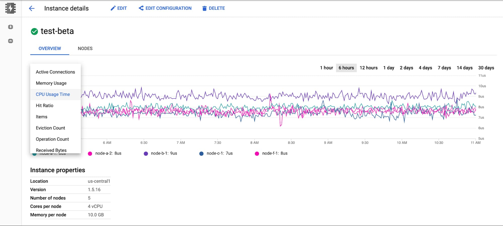
The beta launch is available in major regions across the U.S., Asia, and Europe, and will be available globally soon.
Getting started with Memorystore for Memcached
To get started with Memorystore for Memcached, check out the quick start guide. Sign up for a $300 credit to try Memorystore and the rest of Google Cloud. You can start with the smallest instance and when you’re ready, you can easily scale up to serve performance-intensive applications. Enjoy your exploration of Google Cloud and Memorystore for Memcached.
Cloud Bigtable Helps Fraud-detection Company Meet Scalability Demands and Secure Customer Data

7097
Of your peers have already read this article.
3:00 Minutes
The most insightful time you'll spend today!
Editor’s note: Today we are hearing from Jono MacDougall , Principal Software Engineer at Ravelin. Ravelin delivers market-leading online fraud detection and payment acceptance solutions for online retailers. To help us meet the scaling, throughput, and latency demands of our growing roster of large-scale clients, we migrated to Google Cloud and its suite of managed services, including Cloud Bigtable, the scalable NoSQL database for large workloads.
As a fraud detection company for online retailers, each new client brings new data that must be kept in a secure manner and new financial transactions to analyze. This means our data infrastructure must be highly scalable and constantly maintain low latency. Our goal is to bring these new organizations on quickly without interrupting their business. We help our clients with checkout flows, so we need latencies that won’t interrupt that process—a critical concern in the booming online retail sector.
We like Cloud Bigtable because it can quickly and securely ingest and process a high volume of data. Our software accesses data in Bigtable every time it makes a fraud decision. When a client’s customer places an order, we need to process their full history and as much data as possible about that customer in order to detect fraud, all while keeping their data secure. Bigtable excels at accessing and processing that data in a short time window. With a customer key, we can quickly access data, bring it into our feature extraction process, and generate features for our models and rules. The data stays encrypted at rest in Bigtable, which keeps us and our customers safe.
Bigtable also lets us present customer profiles in our dashboard to our client, so that if we make a fraud decision, our clients can confirm the fraud using the same data source we use.

We have configured our bigtable clusters to only be accessible within our private network and have restricted our pods access to it using targeted service accounts. This way the majority of our code does not have access to bigtable and only the bits that do the reading and writing have those privileges.
We also use Bigtable for debugging, logging, and tracing, because we have spare capacity and it’s a fast, convenient location.
We conduct load testings against Bigtable. We started at a low rate of ~10 Bigtable requests per second and we peaked at ~167000 mixed read and write requests per second at absolute peak. The only intervention that was done to achieve this was pressing a single button to increase the number of nodes in the database. No other changes were made.
In terms of real traffic to our production system, we have seen ~22,000 req/s (combined read/write) on Bigtable in our live environment as a peak within the last 6 weeks.
Migrating seamlessly to Google Cloud
Like many startups, we started with Postgres, since it was easy and it was what we knew, but we quickly realized that scaling would be a challenge, and we didn’t want to manage enormous Postgres instances. We looked for a kind of key value store, because we weren’t doing crazy JOINS or complex WHERE clauses. We wanted to provide a customer ID and get everything we knew about it, and that’s where key value really shines.
I used Cassandra at a previous company, but we had to hire several people just for that chore. At Ravelin we wanted to move to managed services and save ourselves that headache. We were already heavy users and fans of BigQuery, Google Cloud’s serverless, scalable data warehouse, and we also wanted to start using Kubernetes. This was five years ago, and though quite a few providers offer Kubernetes services now, we still see Google Cloud at the top of that stack with Google Kubernetes Engine (GKE). We also like Bigtable’s versioning capability that helped with a use case involving upserts. All of these features helped us choose Bigtable.
Migrations can be intimidating, especially in retail where downtime isn’t an option. We were migrating not just from Postgres to Bigtable, but also from AWS to Google Cloud. To prepare, we ran in AWS like always, but at the same time we set up a queue at our API level to mirror every request over to Google Cloud. We looked at those requests to see if any were failing, and confirmed if the results and response times were the same as in AWS. We did that for a month, fine tuning along the way.
Then we took the big step and flipped a config flag and it was 100% over to Google Cloud. At the exact same time, we flipped the queue over to AWS so that we could still send traffic into our legacy environment. That way, if anything went wrong, we could fail back without missing data. We ran like that for about a month, and we never had to fail back. In the end, we pulled off a seamless, issue-free online migration to Google Cloud.
Flexing Bigtable’s features
For our database structure, we originally had everything spread across rows, and we’d use a hash of a customer ID as a prefix. Then we could scan each record of history, such as orders or transactions. But eventually we got customers that were too big, where the scanning wasn’t fast enough. So we switched and put all of the customer data into one row and the history into columns. Then each cell was a different record, order, payment method, or transaction. Now, we can quickly look up the one row and get all the necessary details of that customer. Some of our clients send us test customers who place an order, say, every minute, and that quickly becomes problematic if you want to pull out enormous amounts of data without any limits on your row size. The garbage collection feature makes it easy to clean up big customers.
We also use Bigtable replication to increase reliability, atomicity, and consistency. We need strong consistency guarantees within the context of a single request to our API since we make multiple bigtable requests within that scope. So within a request we always hit the same replica of Bigtable and if we have a failure, we retry the whole request. That allows us to make use of the replica and some of the consistency guarantees, a nice little trade-off where we can choose where we want our consistency to live.https://www.youtube.com/embed/0-eH5u7rrQQ?enablejsapi=1&
We also use BigQuery with Bigtable for training on customer records or queries with complicated WHERE clauses. We put the data in Bigtable, and also asynchronously in BigQuery using streaming inserts, which allows our data scientists to query it in every way you can imagine, build models, and investigate patterns and not worry about query engine limitations. Since our Bigtable production cluster is completely separate, doing a query on BigQuery has no impact on our response times. When we were on Postgres many years ago, it was used for both analysis and real time traffic and it was not the optimal solution for us. We also use Elasticsearch for powering text searches for our dashboard.
If you’re using Bigtable, we recommend three features:
- Key visualizer. If we get latency or errors coming back from Bigtable, we look at the key visualizer first. We may have a hotkey or a wide row, and the visualizer will alert us and provide the exact key range where the key lives, or the row in question. Then we can go in and fix it at that level. It’s useful to know how your data is hitting Bigtable and if you’re using any anti-patterns or if your clients have changed their traffic pattern that exacerbated some issue.
- Garbage collection. We can prevent big row issues by putting size limits in place with the garbage collection policies.
- Cell versioning. Bigtable has a 3d array, with rows, columns, and cells, which are all the different versions. You can make use of the versioning to get history of a particular value or to build a time series within one row. Getting a single row is very fast in Bigtable so as long as you can keep the data volume in check for that row, making use of cell versions is a very powerful and fast option. There are patterns in the docs that are quite useful and not immediately obvious. For example, one trick is to reverse your timestamps (MAXINT64 – now) so instead of the latest version, you can get the oldest version effectively reversing the cell version sorting if you need it.
Google Cloud and Bigtable help us meet the low-latency demands of the growing online retail sector, with speed and easy integration with other Google Cloud services like BigQuery. With their managed services, we freed up time to focus on innovations and meet the needs of bigger and bigger customers.
Learn more about Ravelin and Bigtable, and check out our recent blog, How BIG is Cloud Bigtable?
How Connected-Stories Uses BigQuery and AI/ML to Craft Personalized Ad Experiences

4001
Of your peers have already read this article.
4:00 Minutes
The most insightful time you'll spend today!
Editor’s note: The post is part of a series highlighting our awesome partners, and their solutions, that are Built with BigQuery
In the field of producing engaging video content such as ads, many marketers ignore the power of data to improve their creative efforts to meet the consumers’ need for personalized messages. The demand for creative tech to efficiently personalize is real as marketers need personalized video Ads to reach their audience with the right message at the right time. Data, Insights and Technology are the main ingredients to deliver this value while ensuring security and privacy requirements are met. The Connected-Stories team partnered with Google Cloud to build a platform for Ad personalization. Google Data Cloud and BigQuery are at the forefront to assimilate data, leverage ML models, create personalized ads, and capitalize on real-time intelligence as the core features of the Connected-Stories NEXT platform.
Connected-Stories NEXT is an end-to-end creative management platform to develop, serve, and optimize interactive video and display ads that scale across any channel. The platform ingests first-party data to create custom ML models, measure numerous third-party data points to help brands develop unique customer journeys and create videos that their data signals can drive. An intelligent feedback loop passes real-time data back, enabling brands to make data-driven and actionable video ads that take the brand’s campaigns to the next level.
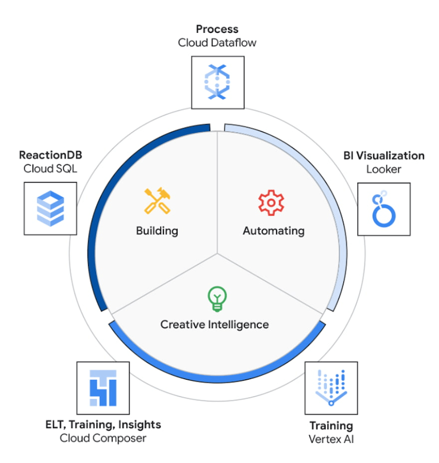
The core use case of the NEXT platform revolves around collecting user’s interaction data and optimizing for precision and speed to create an actionable Ad experience that is personalized for each user. The platform processes complex data points to create interactive data visualizations that allow for accurate analysis. The platform uses Vertex AI to access managed tools, workflows, and infrastructure to build, deploy, and scale ML models that have improved the accuracy to identify segments for further analysis.
The platform ingests 200M data events with peaks and valleys of activity. These events are processed to generate dashboards that enable users to visualize metrics based on filters in real-time. These dashboards have high performance requirements in terms of a responsive user interface under constantly changing data dimensions.
Google Cloud’s serverless stack coupled with limitless data cloud infrastructure has been the core to the NEXT platform’s data-driven innovation. The growing volume of data ingested, streamed and processed were scaled uniformly across the compute, storage and analytical layers of solution. A lean development team at Connected-Stories were able to focus all-in on the solution, while the serverless stack scaled, lowered attack service in terms of security and optimized the cost footprint through pay-as-you-go features.
BigQuery has been the backbone to support the vast amounts of data spreading over multiple geos resulting in workloads running at petabyte scale. BigQuery’s fully managed serverless architecture, real-time streaming, built-in machine learning and rich business intelligence capabilities distinguishes itself from a cloud data warehouse. It is the foundation needed to approach data and serve users in an unlimited number of ways. For an application with zero tolerance for failure, given its fully managed nature, BigQuery handles replication, recovery, data distributed optimization and management.
The platform’s requirements include the need for low maintenance, constantly ingesting and refreshing data and smart-tuning of aggregated data. These capabilities can be implemented by BigQuery’s materialized views feature. Materialized views are useful for precomputed views that regularly cache query results for better performance. These views possess the innate feature to read only the delta change from base tables and calculate the up-to-date aggregations. Materialized views impart faster outputs and consume fewer resources while reducing the cost footprint.
Some key considerations in using Google cloud and focusing on the Serverless stack include: quick onboarding to development, prototyping in short sprints and ease of preparing data in a rapidly changing environment. Typical considerations around low code / no code include data transformation, aggregation and reduced deployment time. These considerations are fulfilled through using serverless capabilities within Google Cloud such as PubSub, Cloud Storage, Cloud Run, Cloud Composer, Dataflow and BigQuery as described in the Architecture diagram below. The use of each of these components and services are described below.
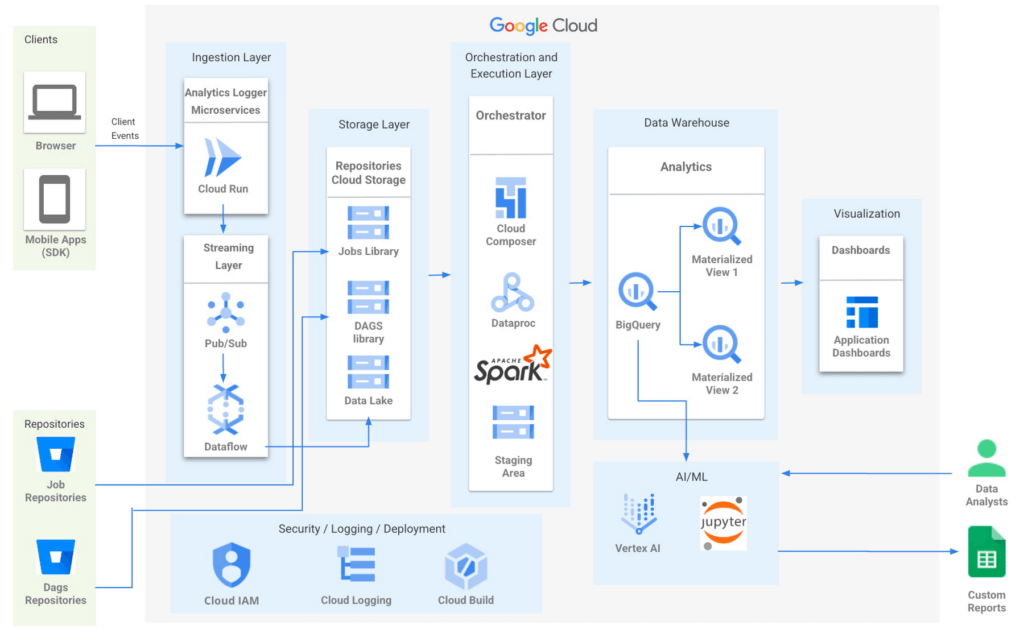
- Input/Ingest: At a high-level, microservices hosted in Cloud Run collect and aggregate incoming Ads events.
- Enrichment: The output of this stage is a Pub-Sub message enriched with more attributes based on a pre-configured campaign.
- Store: a Cloud Dataflow streaming job to create text files in Cloud Storage buckets.
- Trigger: Cloud Composer triggers the spark jobs based on text files to process and group them to produce desired output as one record per impression, a logical group of events.
- Deploy: Cloud Build is then used to automate all deployments.
Thus far, all Google cloud managed services work together to ingest, store and trigger the orchestration, all of which are scalable based on configurations including autoscaling capabilities.
- Visualization: A visualization tool reads data from BigQuery to compute pre-aggregations required for each dashboard.
- Data Model Evolution considerations: Though the solution served the purpose of creating pre-aggregations, as the data model evolved by adding a column or creating a new table, it led to recreating pre-aggregations and querying the data again. Alternatively, creating aggregate tables as an extra output of current ETLs seemed like a viable option. However, this would increase the cost and complexity of jobs. A similar situation to reprocess or update aggregated tables would occur as data is updated.
Precomputed views of data that is periodically cached are critical to reach the audience with the right message at the right time.
- Performance: In order to increase the performance of the platform, we need to have regularly precomputed views of the data, cached .
- Materialized Views: Consumers of these views needed faster response times, to consume fewer resources and output only the changes in comparison to a base table. BigQuery Materialized views were used to solve this very requirement. Materialized views have been highly leveraged to optimize the design resulting in lesser maintenance and access to fresh data with high performance with a relatively low technical investment in creating and maintaining SQL code.
- Dashboards: Application dashboards pointing to the Materialized views are highly performant and provide a view into fresh data.
- Custom Reports with Vertex AI Notebooks: Vertex AI notebooks directly read data from BigQuery to produce custom reports for a subset of customers. Vertex AI has been hugely beneficial to data analysts, where an environment with pre-installed libraries simplifies the readiness to use. Vertex AI Workbench notebooks are used to share these reports within the team allowing them to work always on the cloud without having the need to download data at any time. Besides, it increases the velocity to develop and test ML models faster.
The NEXT platform has yielded benefits such as customers having the ability to create unique consumer journeys powered by AI / ML personalization triggers, using first-party data and business intelligence tools to capitalize on real-time creative intelligence, which is a dashboard to measure campaign performance for cross-functional teams to analyze the impact of Ad content experience at a granular level. All of these while ensuring controlled access to data to enrich data without moving across clouds. The NEXT platform can keep up with increased demands for agility, scalability and reliability through the underlying usage of Google Cloud.
Partnering with Google, in the context of the Google Built with BigQuery program has surfaced the differentiated value in areas of creating interactive personalized Ads by using real-time data. In addition, by sharing this data across organizations as assets, ML models have fueled higher levels of innovation. Connected-Stories plan to deepen the penetration into the entire spectrum of services offered in the AI/ML area to enhance core functionality and provide newer capabilities to the platform.
Click here to learn more about Connected-Stories NEXT Platform capabilities.
The Built with BigQuery Advantage for ISVs
Through Built with BigQuery, launched in April ‘22 as part of Google Data Cloud Summit, Google is helping tech companies like Connected-Stories co-innovate in building applications that leverage Google’s data cloud with simplified access to technology, helpful and dedicated engineering support, and joint go-to-market programs. Participating companies can:
- Get started fast with a Google-funded, pre-configured sandbox.
- Accelerate product design and architecture through access to designated technical experts from the ISV Center of Excellence who can share insights from key use cases, architectural patterns, and best practices encountered in the field.
- Amplify success with joint marketing programs to drive awareness, generate demand, and increase adoption.
The Google Data Cloud spectrum of products and specifically BigQuery give ISVs the advantage of a powerful, highly scalable data warehouse that’s integrated with Google Cloud’s open, secure, sustainable platform. And with a huge and expanding partner ecosystem and support for multi-cloud, open source tools and APIs, Google provides technology companies the portability and extensibility they need to avoid data lock-in and exercise choice.
We thank the Google Cloud and Connected-Stories team members who co-authored the blog: Connected-Stories: Luna Catini, Marketing Director, Google: Sujit Khasnis, Cloud Partner Engineering
More Relevant Stories for Your Company

Developers and Practitioners’ Guide for Moving On-prem Data Warehouse to BigQuery
Data teams across companies have continuous challenges of consolidating data, processing it and making it useful. They deal with challenges such as a mixture of multiple ETL jobs, long ETL windows capacity-bound on-premise data warehouses and ever-increasing demands from users. They also need to make sure that the downstream requirements

Move over Myths! Here’s What You Need to Know about Cloud Spanner
Intro to Cloud Spanner Cloud Spanner is an enterprise-grade, globally distributed, externally consistent database that offers unlimited scalability and industry-leading 99.999% availability. It requires no maintenance windows and offers a familiar PostgreSQL interface. It combines the benefits of relational databases with the unmatched scalability and availability of non-relational databases. As organizations




Crux Accelerates Data Operations with Google BigQuery
Being in the constantly evolving and changing data business, Crux Informatics has integrated with Google Cloud and BigQuery to achieve the benefits of a data cloud, including fully managed global scale, load management, high performance, and genuinely good support. Watch this video to learn more about how this partnership will

Query Insights for Spanner: A blessing for developers and DBAs
Today, application development teams are more agile and are shipping features faster than ever before. In addition to these rapid development cycles and the rise of microservices architectures, the end-to-end ownership of feature development (and performance monitoring) has moved to a shared responsibility model between advanced database administrators and full-stack
