





BigQuery Reference Guide: Understanding Tables within and Routine for Data Transformation

3686
Of your peers have already read this article.
3:00 Minutes
The most insightful time you'll spend today!
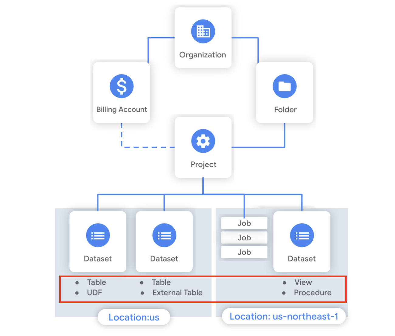
Last week in our BigQuery Reference Guide series, we spoke about the BigQuery resource hierarchy – specifically digging into project and dataset structures. This week, we’re going one level deeper and talking through some of the resources within datasets. In this post, we’ll talk through the different types of tables available inside of BigQuery, and how to leverage routines for data transformation. Like last time, we’ll link out to the documentation so you can learn more about using these resources in practice.
What is a table?
A BigQuery table is a resource that lives inside a dataset. It contains individual records organized into rows, with each record composed of columns (also called fields) where a specified data type is enforced. BigQuery supports numerous different data types including GEOGRAPHY for geospatial data, STRUCT and ARRAY for more complex data, and new parameterized data types to add specific constraints like the number of characters in a string.
Data access can also be controlled at the table, row and column levels; more details on data governance will be covered later in the series. Metadata, such as descriptions and labels, can be used for surfacing information to end users and as tags for monitoring. You can create and manage a table directly in the UI, through the API / Client SDKs or in a SQL query using a DDL statement.
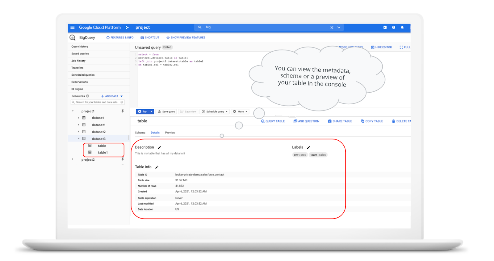
bq show \--schema \--format=prettyjson \project1:dataset3.table
Managed and external tables
Managed tables are tables that are backed by native BigQuery storage, which has many benefits that improve query performance including support for partitions and clusters. We’ll cover more details on BigQuery storage later in this series. Another advantage of using a managed table is that BigQuery allows you to use time travel to access data from any point within the last seven days and query data that was updated, expired or deleted. And now you can even create a snapshot of your table, to preserve its contents at a given time.
# create a snapshot of transactions in the library_backup dataset as of one hour agoCREATE SNAPSHOT TABLElibrary_backup.salesCLONE retail.transactionsFOR SYSTEM_TIME AS OF TIMESTAMP_SUB(CURRENT_TIMESTAMP(), INTERVAL 1 HOUR);
While managed tables store data inside BigQuery storage, external tables are backed by storage external to BigQuery. BigQuery currently supports creating an external table from Cloud Storage, Cloud Bigtable and Google Drive. Besides an external table, you can create a connection to Cloud SQL, which is somewhat analogous to an external dataset. Here, you can leverage federated queries to send a query that executes in Cloud SQL but returns the results to be used within BigQuery.
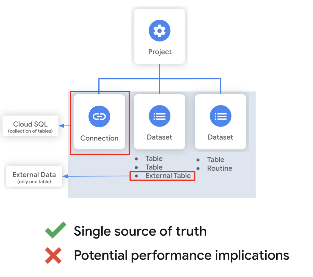
Using external tables or federated queries may result in queries that aren’t as fast as if the data had been stored in BigQuery itself. However, they can be useful for some data transformation patterns – for example, you may want to schedule a DDL/DML query that hydrates a managed table using a federated query, which selects and transforms data from Cloud SQL. An external table might also be useful for multi-consumer workflows where BQ storage isn’t the source of truth. Like, if you have a dataproc cluster accessing data in a Cloud Storage bucket that you’re not quite ready to port into BigQuery (although I do recommend taking a look at our connector if you need some convincing). You can learn more about querying external data in this video.
Logical and materialized views
In BigQuery, you can create a virtual table with a logical view or a materialized view. With logical views, BigQuery will execute the SQL statement to create the view at run time, it will not save the result anywhere. Additionally, you can grant users access to an authorized view to share query results without giving them access to the underlying tables.
# create a view that aggregates daily sales from a retail transaction tableCREATE VIEW retail.daily_sales as (SELECT date(t.transaction_timestamp) as date, sum(li.sale_price) as total_salesFROM retail.transaction_detail as tLEFT JOIN UNNEST(t.line_items) as liGROUP BY 1)
On the other hand, materialized views are re-computed in the background when the base data changes. No user action is required – they are always fresh! Better yet, if a query, or part of a query, against the source table can be resolved by querying the materialized view, BigQuery will reroute for improved performance. However, materialized views use a restricted SQL syntax and a limited set of aggregation functions. You can find details on limitations here.
# create a materialized view that aggregates daily salesCREATE MATERIALIZED VIEW retail.daily_sales as (SELECT date(t.transaction_timestamp) as date, sum(li.sale_price) as total_salesFROM retail.transaction_detail as tLEFT JOIN UNNEST(t.line_items) as liGROUP BY 1)
Temporary and cached results tables
Aside from the tables we’ve mentioned so far, you can also create a temporary managed table using the TEMP or TEMPORARY keyword. This table is saved in BigQuery storage and can be referenced for the duration of the script. Temporary tables can be a good alternative to WITH clauses because the defining query is only executed once as opposed to being inlined every place the alias is referenced.
| Original code | Optimized |
| with a as ( select …),b as ( select … from a …),c as ( select … from a …)select b.dim1, c.dim2from b, c; | create temp table a asselect …; with b as ( select … from a …),c as ( select … from a …)select b.dim1, c.dim2from b, c; |
It’s also important to mention that BigQuery writes all query results to a table – one either explicitly identified by the user or to a cached results table. Temporary, cached results tables are maintained per-user, per-project. There are no storage costs for temporary tables.
User defined functions & procedures
In BigQuery, a routine is either a user defined function (UDF) or a procedure. Routines allow you to re-use logic and handle your data in a unique way. A UDF is a function that is created using either SQL or Javascript, it takes arguments as input and returns a single value as an output. UDFs are often used for cleaning or re-formatting data. For example, extracting parameters from a URL string, restructuring nested data, or cleaning up strings:
# UDF to clean up string valuesCREATE OR REPLACE FUNCTIONmy_dataset.cleanse_string_test (text STRING)RETURNS STRINGAS (REGEXP_REPLACE(LOWER(TRIM(text)), '[^a-zA-Z0-9 ]+', ''));
We even have a community driven open-source repository of BigQuery UDFs! Just like logical views, you can create an authorized UDF that protects aspects of the underlying data. For more details on UDFs checkout our video here. You might also want to take a look at table functions – a preview feature where you can create a SQL UDF that returns a table instead of a scalar value.
Procedures, on the other hand, are blocks of SQL statements that can be called from other queries. Unlike UDFs, stored procedures can return multiple values or no values – which means you can run them to create or modify tables. In BigQuery, you can also leverage scripting capabilities within procedures to control execution flow with IF and WHILE statements. Plus, you can call your UDFs within your procedure! These aspects make procedures great for extract-load-transform (ELT) driven workflows.
# Procedure to create daily sales rollup, starting from startDate until endDateCREATE OR REPLACE PROCEDURE my_dataset.sum_sales(startDate STRING, endDate STRING)BEGINCREATE OR REPLACE TABLE retail.sales_resultAS (SELECTdate(t.transaction_timestamp) as date,sum(li.sale_price) as total_salesFROM retail.transaction_detail as tLEFT JOIN UNNEST(t.line_items) as liWHERE transaction_timestamp >= TIMESTAMP(startDate) AND transaction_timestamp <= TIMESTAMP(endDate)GROUP BY 1);END;CALL retail.sum_sales('2020-08-01', '2020-01-20');
To ensure consistent analytics across your organization, I recommend that you create a library dataset to house UDFs and procedures. You can easily grant everyone in your organization the BigQuery Data Viewer role to the library dataset so that all analysts use consistent and up-to-date logic in their queries.
Stay tuned!
We hope this gave you an understanding of how to leverage some of the different resources inside of a BigQuery dataset, and to help you make decisions like using native versus external storage, logical versus materialized views, and user defined functions or procedures.
Next up we’ll be talking about workload management in BigQuery by taking a look at jobs and the reservation model. Be sure to keep an eye out for more in this series by following me on LinkedIn and Twitter, and subscribing to our Youtube channel.
How Pantheon Improved Performance and Reliability by Moving to Google Cloud

5589
Of your peers have already read this article.
1:30 Minutes
The most insightful time you'll spend today!
Google Cloud Results
- Improves performance and reliability, enabling Pantheon to serve larger customers
- Supports 99.95% uptime across 200,000+ websites
- Reduces cloud infrastructure costs by 40%
- Enables future analytics offerings based on machine learning and big data analytics
Nearly every business needs a web presence—but the vast majority of companies don’t want to be involved in the technical aspects of coding, deployment, hosting, security, and scaling websites. To stay focused on the business value and creative aspects of their websites and avoid managing infrastructure, thousands of companies turn to Pantheon, a website operations and hosting platform that powers over 200,000 websites.
Pantheon promises its customers speed, reliability, and scalability plus world-class collaboration and workflow tools. For five years, the company was able to deliver high service levels in all three areas running its platform on bare-metal virtual cloud servers. However, as its business grew, network links began to saturate under heavy load, risking instability. As Pantheon’s business evolved to focus on servicing some of the largest websites in the world, the company wanted to partner with a more innovative cloud services provider.
“We wanted a partner that could give us what we offer to our own customers: the flexibility to scale smoothly and consume services without building them from scratch,” says David Strauss, CTO, Pantheon. “It was time to move beyond custom containers on managed VMs and extend our cloud strategy to include next-generation technologies for container management and analytics.”
Pantheon evaluated several leading cloud providers and determined that Google Cloud Platform would be the best fit for its business and customers. Engineering had the final say, running a battery of functionality and performance tests at the storage, database, and web server layers.
“In every test our engineers did, Google Cloud Platform came in as better, faster, and more cost effective than the competition,” says Niall Hayes, COO, Pantheon. “We compared MariaDB to Google Cloud SQL and Cassandra to Google Bigtable, and container density improved from 250 to 400 containers per server.”
Migrating 200,000+ sites in 2 weeks
Pantheon wanted to make the transition transparent to its customers, so a fast and smooth migration to Google Cloud Platform was essential. With help from Google, Pantheon completed the migration quickly and moved 500TB of databases, code, and files with zero customer impact.
“We migrated over 200,000 websites to Google Cloud Platform in 2 weeks, including 50,000 that are heavily trafficked and actively developed, and nobody noticed,” says Josh Koenig, Co-founder and Head of Products at Pantheon. “The speed was incredible. There was no downtime, and we filed no additional support tickets with Google during the entire process.”
The platform for platforms
For its content management system runtime environment, Pantheon runs its own homegrown container management technology on Google Compute Engine. To automate scaling for other core services such as its routing layer and distributed file system, it uses Google Kubernetes Engine for cluster management and orchestration.
“Google is the clear leader in Kubernetes and container management, which aligns very well with our open source values and our vision for the future,” says Niall. “With Google Kubernetes Engine we get better resource efficiency, and automated operations and autoscaling take a lot of administration off our plate.”
In addition to smooth scaling, Pantheon and its customers benefit from improved performance and reliability thanks to the high-quality private network offered by Google.
Further, the Google partnership with Fastly enables direct connectivity to Google Cloud Platform to improve performance for edge caching. As a result of these improvements, Pantheon raised its availability service level agreement (SLA) from 99.9% to 99.95% and can now take on even larger customers.
“Google’s network topology, both locally and globally, performs better and more reliably than competing solutions, making Google Cloud Platform the best choice for us and for our customers,” says David. “Google beats any other cloud provider as the best platform-for-platforms.”
Adds Josh: “Google has unbelievable technology around persistence and replication between zones and regions, and that is not something we could find anywhere else. This allows us to offer advanced disaster recovery and failover services to our customers.”
Strengthening customer relationships
Pantheon uses Google BigQuery, a fully managed, cloud-based data warehouse, to integrate with Fastly and analyze website traffic on behalf of its customers. Previously, Pantheon was unable to ingest edge data quickly enough from Fastly, limiting its ability to identify issues and provide the best customer service. Today, Fastly streams logs in real time into Google BigQuery for analysis, giving Pantheon a wealth of insights.
“We use Google BigQuery to identify customers that have outgrown their infrastructure or need to right-size for business growth,” says David. “We can have proactive conversations and add a lot of value to the relationships. Soon, we plan to make Google BigQuery available to our customers so they can better understand their own traffic.”
Adds Niall: “Google Cloud Platform is more data-oriented than other cloud providers, making it a better match for our needs and our customers’ strategic initiatives.”
Integrated, granular security
Pantheon appreciates that Google Cloud services are built for public cloud, with granular security as a core design and development requirement. Employees simply use their G Suite credentials to gain access to Google Cloud Platform infrastructure and services.
“We’ve been a G Suite shop for years because of the paperless collaboration benefits,” says Josh. “G Suite connects our distributed company, and it was very natural to use those same logins for Google Cloud Platform.”
Staying competitive and productive
Moving to Google Cloud Platform opens up new possibilities for services Pantheon can offer to customers in the future, including machine learning and big data analytics, to give them a more complete view of how digital experiences are driving their businesses. Internally, engineers can move faster, do more effective capacity planning, and provide better service as Pantheon moves its products upmarket.
Pantheon expected to save 20% on cloud infrastructure costs by moving to Google Cloud Platform, but was able to double that savings with resource optimization and managed services.
“Since moving to Google Cloud Platform, our platform is more secure, reliable, and scalable than ever. We reduced our cloud infrastructure costs by 40%, and our customers’ sites run 45% faster than industry benchmarks,” says Niall. “Our engineers are Google fans for a reason—they’re happier, more efficient, and more productive on Google Cloud Platform.”
Discover Effingo: Google’s Solution to Moving Data at Massive Scale

1358
Of your peers have already read this article.
3:30 Minutes
The most insightful time you'll spend today!
Every hour of every day, Google moves a lot of data around the world. But how? With the Effingo (Latin for ‘to duplicate’ or ‘copy’) data copying service, a Google-only service that moves data internally and on Google Cloud customers’ behalf.
As a Google Cloud customer perhaps you move data with Storage Transfer Service, a managed transfer option that provides out-of-the-box security, reliability, and performance, that eliminates the need to optimize and maintain scripts, and handle retries. Storage Transfer Service is useful for consolidating data from separate projects, to move data into a backup location, or to change the location of your data.
Likewise, Google’s internal services need very similar functionality to manage their data. This includes data that is in charge of the ecosystem of Google Cloud services, such as BigQuery and Cloud Spanner.
Effingo solves a challenging problem of data movement at a global scale. It supports a wide range of workloads with different traffic characteristics and different requirements for data replication, durability, and latency. In this article we will explore the main motivations behind data movement and solutions to core infrastructure problems that we face when copying exabytes of data on a daily basis.
Why move data in the first place?
But first, let’s think about why you even want to move or geographically distribute your data.
For one thing, you want to replicate your data for durability and reliability. You definitely don’t want to keep a single copy of your data. In the end, we’re talking about a file that is stored on a hard drive. Any hard drive can fail at any point. For this reason, keeping copies of your data in different locations helps ensure that at any point of time there is a copy of your file that you can read from. Moreover, these locations should be geographically distant from each other to avoid even temporary data loss due to natural disasters, network cuts, and other incidents that can impact a local area.
Second, you want your data to be close to your users to reduce latency. You want to serve data with minimal delay to give a great user experience. In many cases, delays caused by data transfers from remote locations can spoil the usability of your application or create the perception that your service doesn’t work. According to Google research, 53% of mobile users abandon sites that take over 3 seconds to load. There are other consequences of lack of data proximity: for example, transferring data from distant locations wastes network resources, which can have a negative impact on the environment. Google has been carbon-neutral for our operations since 2007, and we have matched 100% of the electricity consumption of our operations with renewable energy purchases annually since 2017, but we aim higher: Our goal is to run all our data centers and offices on carbon-free energy, 24/7, by 2030.
The third reason to geographically distribute your data is to balance storage capacity between clusters. This reduces the cost of storing data because it enables us to increase the overall capacity of our data centers and use computation power in less loaded clusters. We can then limit the amount of wasted resources and use otherwise idle hardware. This is especially relevant for batch processing and storing cold data where the exact storage location is not that important.
What are the challenges?
Operating at such a large scale as Google makes data movement a challenging problem for several reasons. Here are a few examples.
Data must be secure and consistent at its destination. Achieving this is complex. For example, to copy a file from one location to another, you need the following: throughput to read and write to disks, network capacity to transfer bytes between data centers, and compute resources to instrument the whole operation.
Considering the volume of data that Google operates on, high and predictable throughput is one of the key features of a copy service at scale. It is typical to transfer terabytes of data per second, and so it’s essential to have a scalable service that can handle traffic with sometimes rapidly changing patterns. It poses a further question: how to run such a service and still be resource efficient?
Finally, it’s crucial to ensure high system availability. Google infrastructure is dynamic and copying data between any two clusters may behave differently at different points of time. Effingo needs to be resilient to cluster turndowns, network bottlenecks, rapid changes in resource demands and capacity, and so on.
How do we solve (some) of these problems?
One of the core use cases for data movement is replication. If you want to ensure that your data is reliable, you want to keep more than one copy, ideally in different locations, to be less prone to data loss.
Let’s consider the following example. You have a file in cluster A, and you want to make copies in destinations B – G.
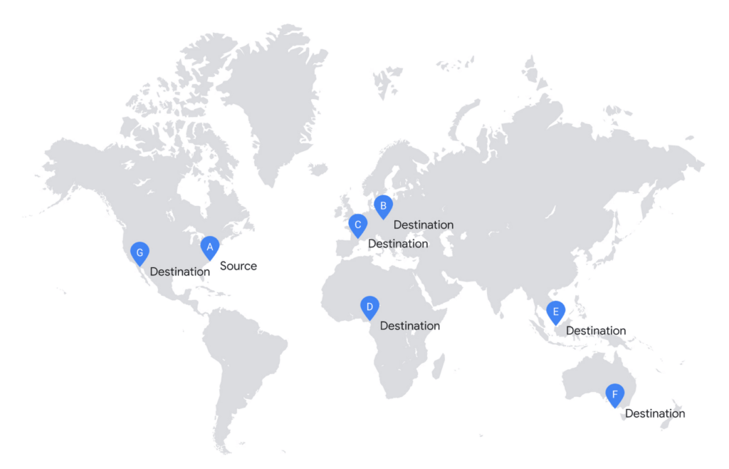
In the simplistic approach, you would start copying to all destinations in parallel.
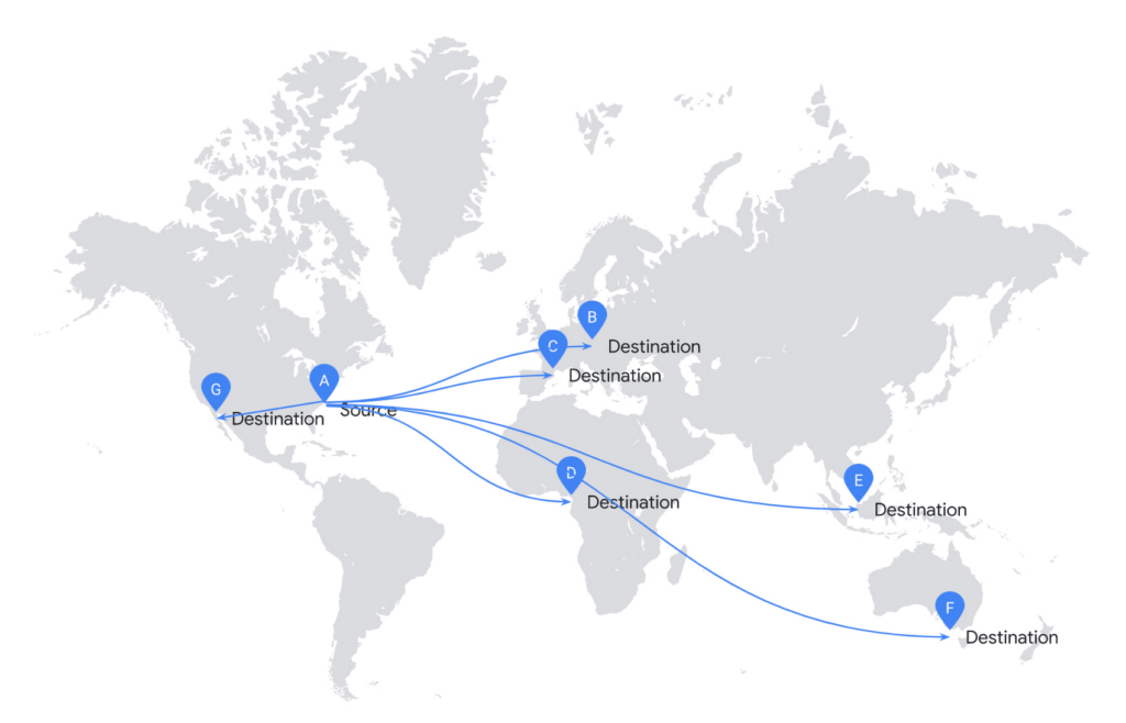
Unfortunately, it is highly inefficient to replicate your file this way. This solution doesn’t scale and requires significant investment in infrastructure.
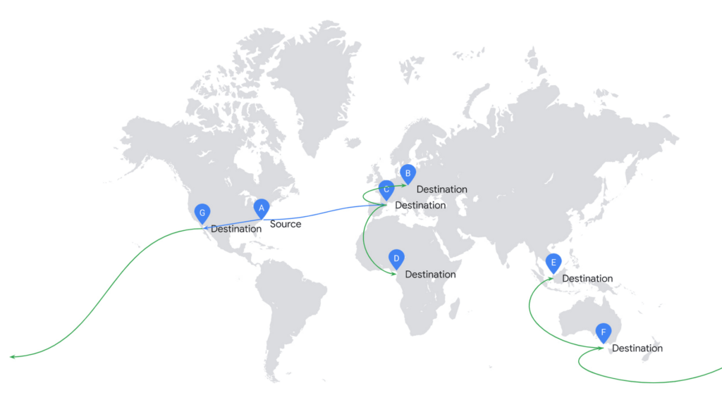
If you consider the cost of network infrastructure, moving data across the ocean is an expensive operation. Effingo creates data transfer plans that reduce the volume of data to transfer across the ocean. If possible, it reuses already replicated data as a new source.
To create data transfer plans Effingo needs to know alternative data sources and be aware of the network topology.
If it goes to the alternative sources, Effingo stores a recent history of transferred files together with their metadata and time-bound permissions to access the files. Whenever a new copy is issued, Effingo checks whether there were copies of the original file that could serve as the same source but in the alternative location. Worth noting is that Effingo is very strict in verifying that both files — the requested source file and the alternative transfer file — are indeed the same to follow high security standards. Effingo not only checks whether the same user issued a copy from the same source but also if file properties including checksum, ciphertext checksum, mtime and several others match.
Once Effingo knows the source files and their alternative sources, it creates a transfer plan over the Google network. Effingo has a model of the network in the form of a graph where each location is a node and each edge is a weighted link between each node. For each copy Effingo creates a Minimum Spanning Tree over such a graph, which serves as an input to the transfer engine. Thanks to this approach we can select a plan that is optimal for each copy.
In the next example, we show a more efficient approach. Effingo first makes an expensive copy to a remote location and then uses it as a new source. For instance, Effingo first copies a file from the US (source A) to Europe (destination C) and then uses the Europe-based file as a copy source for copies on the same continent. Note that Effingo never stores files in temporary locations for optimization purposes – the service only uses locations explicitly requested by our users.
In addition to resource efficiency, the main challenge is to ensure high throughput of data transfer. We solve this problem by applying several approaches that address different problems that may arise.
As described above, our customers’ workloads exhibit a range of different traffic patterns, which results in dynamic changes in capacity on each network link. For this reason, Effingo not only needs to respond to altering resource availability, but also to ensure user fairness in such conditions. In other words, Effingo wants all copy operations to progress while using resources in the best possible way. To achieve this, it uses sophisticated parallelism controls. These controls scale the service up to meet increased demand and limit service capacity if there is service overload, performance degradation, or resource waste.
Further, Effingo must be very resilient and react quickly to errors. On the file level, the service extensively uses retries for transient failures and aborts transfers quickly if it detects non-retryable errors. Effingo uses metrics, logs, and other observability signals to adjust data transfers when needed. For example, it can detect that copies from a specific source are slow and there is another file replica available. Effingo then reconfigures the copy operation to use the other replica to complete the data move.
Data movement at global scale is hard
Hopefully at this point you have a better understanding of why moving data is a challenging problem for infrastructure that operates at Google’s global scale. Effingo supports a range of services that run on Google infrastructure, including Google Cloud services and many internal Google services. While moving data at large scale requires a lot of attention to resource usage and resilience to support high throughput, there is good news: We keep working on this problem and make our infrastructure better every day, so you can run your business on Google Cloud and all data movement is transparent to you.
Google Cloud Tools Help U.S. Forest Department Generate Years of Insights into Earth’s Natural Resources

5019
Of your peers have already read this article.
3:00 Minutes
The most insightful time you'll spend today!
For 117 years, the U.S. Department of Agriculture’s Forest Service has been a steward of America’s forests, grasslands, and waterways. It directly manages 193 million acres and supports sustainable management on a total of 500 million acres of private, state, and tribal lands. Its impact reaches far beyond even that, offering its research and learning freely to the world.
At Google, we’re big admirers of the Forest Service’s mission. So we were thrilled to learn in 2011 that its scientists were using Google Earth Engine, our planetary-scale platform for Earth Science data and analysis, to aid its research, understanding, and effectiveness. In the years since, Google has worked with the Forest Service to meet its unique requirements for visual information about the planet. Using both historical and current data, the Forest Service built new products, workflows, and tools that help more effectively and sustainably manage our natural resources. The Forest Service also uses Earth Engine and Google Cloud to study the effects of climate change, forest fires, insects and disease, helping them create new insights and strategies.
Besides gaining newfound depths of insight, the Forest Service has also sped up its research dramatically, enabling everyone to do more. Using Google Cloud and Earth Engine, the Forest Service reduced the time it took to analyze 10 years worth of land-cover changes from three months to just one hour, using just 100 lines of code. The agency built new models for coping with change, then mapped these changes over time, in its Landscape Change Monitoring System (LCMS) project.
Emergency responders can now work better on new threats that arise after wildfires, hurricanes, and other natural disasters. Forest health specialists can detect and monitor the impacts of invasive insects, diseases, and drought. More Forest Service personnel can use new tools and products within Earth Engine, thanks to numerous training and outreach sessions within the Forest Service.
Researchers elsewhere also benefited when the Forest Service created new toolkits, and posted them to GitHub for public use. For example, there’s geeViz, a repository of Google Earth Engine Python code modules useful for general data processing, analysis, and visualization.
This is only the start. Recently, the Forest Service started using Google Cloud’s processing and analysis tools for projects like California’s Wildfire and Forest Resilience Action Plan. Forest Service researchers also use Google Cloud to better understand ecological conditions across landscapes in projects like Fuelcast, which provides actionable intelligence for rangeland managers, fire specialists, and growers, and the Scenario Investment Planning Platform for modeling local and national land management scenarios.
The Forest Service is a pioneer in building technology to help us better understand and care for our planet. With more frequent imaging, rich satellite data sets, and sophisticated database and computation systems, we can view and model the Earth as a large-scale dynamic system.
We are honored and excited to respond to the unique set of requirements of the scientists, engineers, rangers, and firefighters of the USFS, and look forward to years of learning about — and better caring for — our most precious resources.
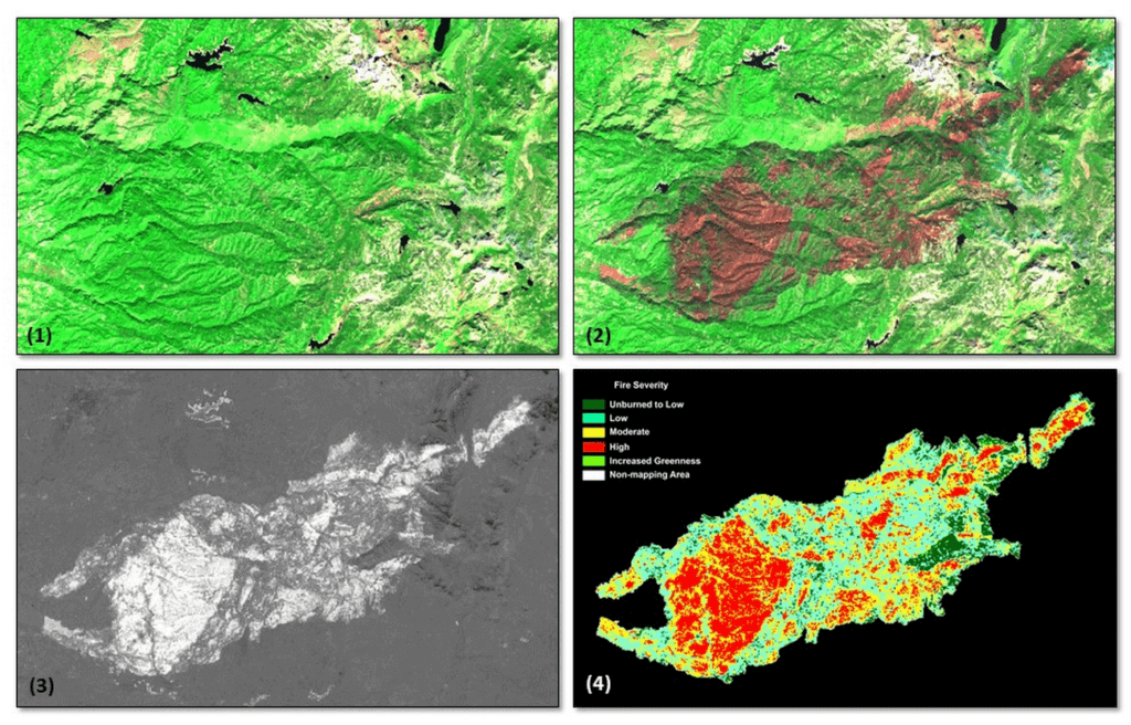
*Image 1: The USDA Forest Service (USFS) Geospatial Technology and Applications Center (GTAC) uses science-based remote sensing methods to characterize vegetation and soil condition after wildland fire events. The results are used to facilitate emergency assessments to support hazard mitigation, to inform post-fire restoration planning, and to support the monitoring of national fire policy effectiveness. GTAC currently conducts these mapping efforts using long-established geospatial workflows. However, GTAC has adapted its post-fire mapping and assessment workflows to work within Google Earth Engine (GEE) to accommodate the needs of other users in the USFS. The spatially and temporally comprehensive coverage of moderate resolution multispectral data sources (e.g., Landsat, Sentinel 2) and analytical power provided by GEE allows users to create geospatial burn severity products quickly and easily. Box 1 shows a pre-fire Sentinel-2 false color composite image. Box 2 shows a post-fire Sentinel-2 false color composite image with the fire scar apparent in reddish brown. Box 3 shows a differenced Normalized Burn Ratio (dNBR) image showing the change between the pre- and post-fire images in Boxes 1 and 2. Box 4 shows a thresholded dNBR image of the burned area with four classes of burn severity (unburned to high severity), which is the final output delivered to forest managers.
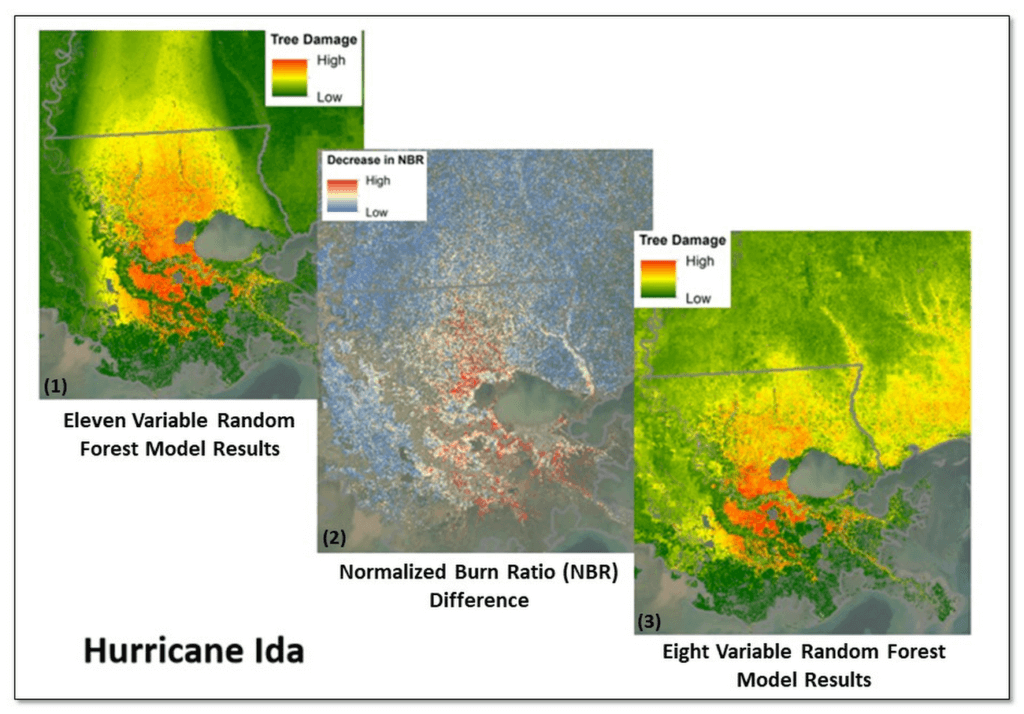
*Image 2: Leveraging Google Earth Engine (GEE), the USDA Forest Service (USFS) Geospatial Technology and Applications Center (GTAC) and USFS Region 8, developed the Tree Structure Damage Impact Predictive (TreeS-DIP) modeling approach to predict wind damage to trees resulting from large hurricane events and produce spatial products across the landscape. TreeS-DIP results become available within 48 hours following landfall of a large storm event to allow allocation of ground resources to the field for strategic planning and management. Boxes 1 and 3 above show TreeS-DIP modeled outputs with varying data inputs and parameters. Box 2 shows changes in greenness (Normalized Burn Ratio; NBR) that was measured with GEE during the recovery from Hurricane Ida and is shown as a visual comparison to the rapidly available products from TreeS-DIP.
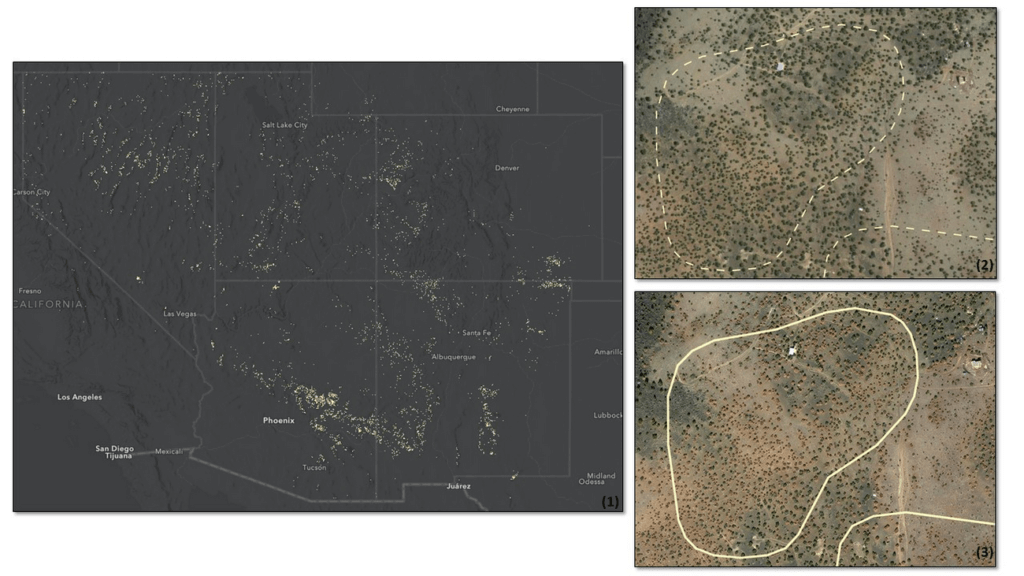
*Image 3: Severe drought conditions across the American West prompted concern about the health and status of pinyon-juniper woodlands, a vast and unique ecosystem. In a cooperative project between the USDA Forest Service (USFS) Geospatial Technology and Applications Center (GTAC) and Forest Health Protection (FHP), Google Earth Engine (GEE) was used to map pinyon pine and juniper mortality across 10 Western US States. The outputs are now being used to plan for future work including on-the-ground efforts, high-resolution imagery acquisitions, aerial surveys, in-depth mortality modeling, and planning for 2022 field season work.
Box 1 contains remote sensing change detection outputs (in white) generated with GEE, showing pinyon-juniper decline across the Southwestern US. Box 2 shows NAIP imagery from 2017 with, with box 3 showing NAIP imagery from 2021. NAIP imagery from these years shows trees changing from healthy and green in 2017 to brown and dying in 2021. In addition, box 2 and box 3 show change detection outputs from Box 1 for a location outside of Flagstaff, AZ converted to polygons (in white). The polygon in box 2 is displayed as a dashed line to serve as a reference, while the solid line in box 3 shows the measured change in 2021. Converting rasters to polygons allows the data to be easily used on tablet computers, as well as the ability to add information and photographs from field visits.
Google Cloud Announces General Availability of BigQuery Row-level Security
6611
Of your peers have already read this article.
3:00 Minutes
The most insightful time you'll spend today!
Data security is an ongoing concern for anyone managing a data warehouse. Organizations need to control access to data, down to the granular level, for secure access to data both internally and externally. With the complexity of data platforms increasing day by day, it’s become even more critical to identify and monitor access to sensitive data. In many cases, sensitive data is co-mingled with non-sensitive data, and access restrictions to sensitive data need to be enabled based on factors like data location or presence of financial information. There may also be nuances where data is sensitive for some groups of users, while for others, it is not.
Today, we’re pleased to announce the general availability of BigQuery row-level security, which gives customers a way to control access to subsets of data in the same table for different groups of users. Row-level security (RLS) extends the principle of least privilege access and enables fine-grained access control policies in BigQuery tables. BigQuery currently supports access controls at the project-, dataset-, table- and column-level. Adding RLS to the portfolio of access controls now enables customers to filter and define access to specific rows in a table based on qualifying user conditions—providing much needed peace of mind for data professionals.
“Our digital transformation and migration of data to the cloud magnifies the business value we can extract from our information assets. However, granular data access control is essential to comply with international regulatory and contractual requirements. BigQuery row-level security helps us comply with data residency and export restrictions,” says Jarrett Garcia, Iron Mountain’s Enterprise Data Platform Senior Director. “It enables us to manage fine-grained access controls without replicating data. What used to take months for approval and access provisioning can now be done more efficiently and effectively. We are looking forward to implementing additional data security capabilities on the BigQuery roadmap to address other critical business use cases.”
How BigQuery row-level security works
Row-level security in BigQuery enables different user personas access to subsets of data in the same table. Customers who are currently using authorized views to enable these use cases can leverage RLS for ease of management. To express the concept of RLS, we have introduced a new entity in BigQuery called row access policy. Row access policies map a group of user principals to the rows that they can see, defined by a SQL filter predicate.
Secure logic rules created by data owners and administrators determines which user can see which rows through the creation of a row-level access policy. The row-level access policies created on a target table by administrators or data owners are applied when a query is run on the table. One table can have multiple policies applied to it.
Below is an example, where row-level access policies have been created to filter data based on users’ “region”.

In the illustrated scenario above, row-level access policies have been created to verify a querying user’s region and to give them access only to the subset of data relevant to that region. Access policies are granted to a grantee list which support all types of IAM principles such as individual users, groups, domains or service accounts. In this example, when a user queries the table, row-level access policies are evaluated to assess which, if any, policies are applicable to that user. The group ‘sales-apac’ is granted access to view a subset of rows where region = ‘APAC’ whereas the group ‘sales-us’ is granted access to view a subset of rows where the region = ’US’. Likewise, users in both groups will see rows in both regions, and users in neither group will not see any rows.
Row-level access policies can also be created using the SESSION_USER() function to restrict access only to rows that belong to the user running the query. If none of the row access policies are applicable to the querying user, the user will have no access to the data in the table.
When a user queries a table with a row-level access policy, BigQuery displays a banner notice indicating that their results may be filtered by a row-level access policy. This notice displays even if the user is a member of the `grantee_list`.

When to put BigQuery row-level security to work
Row-level access policies are useful when you have a need to limit access to data based on filter conditions. The row-access policies’ filter predicate supports arbitrary SQL, and is conceptually similar to the WHERE clause of a SQL query. Filter predicates support the SESSION_USER() function to restrict access only to rows that belong to the user running the query. If none of the row access policies are applicable to the querying user, the user will have no access to the data in the table. Currently, the column used for filtering must be in the table, but we anticipate adding support for subqueries in the filter expression, opening up access to use cases where data is filtered based on lookup tables and calculated values. Row-level access policies can be created, updated and dropped using DDL statements. You will be able to see the list of row-level access policies applied to a table using the BigQuery schema pane in the Cloud Console, which simplifies the management of policies per table, or by using the bq command-line tool.
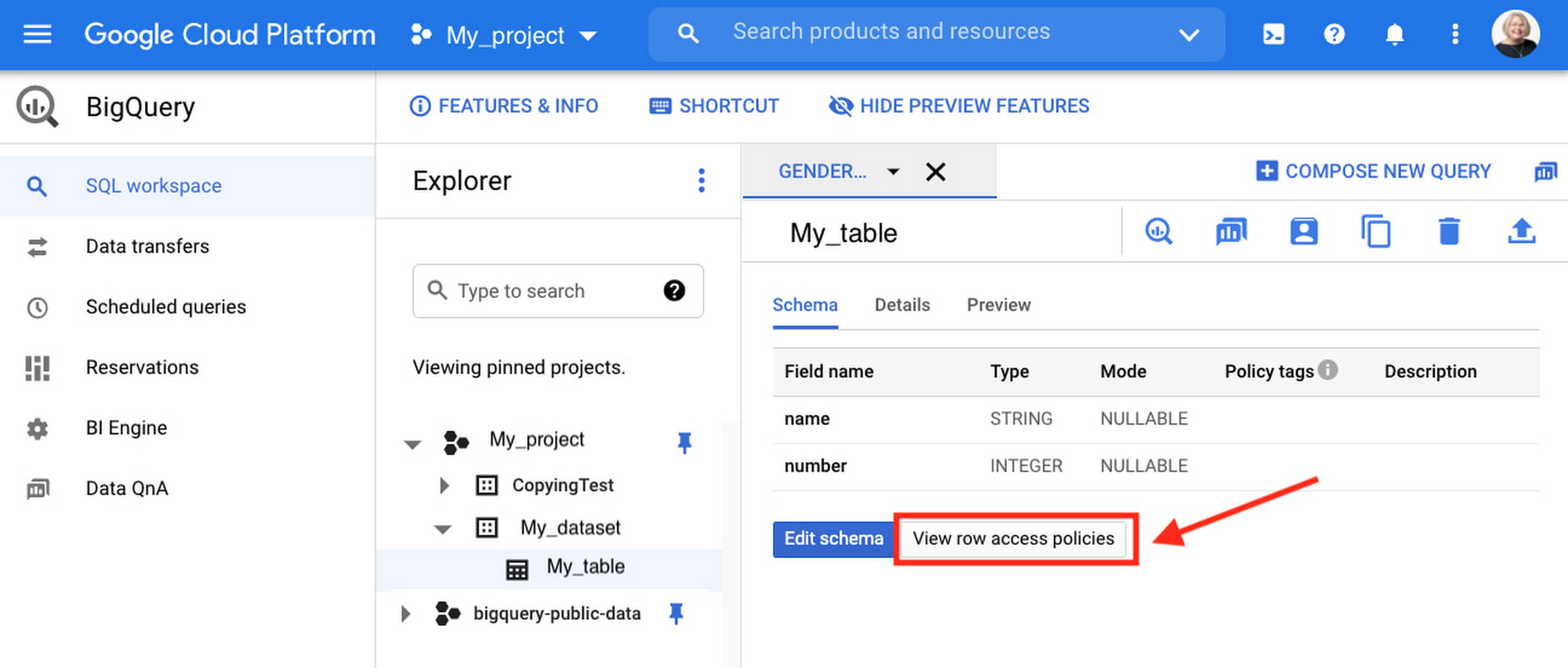
Row-level security is compatible with other BigQuery security features, and can be used along with column-level security for further granularity. Since row-level access policies are applied on the source tables, any actions performed on the table will inherit the table’s associated access policies, to ensure access to secure data is protected. Row-level access policies are applicable to every method used to access BigQuery data (API, Views, etc).
Try it out
We’re always working to enhance BigQuery’s (and Google Cloud’s) data governance capabilities, to provide more controls around managing your data. With row-level security, we are adding deeper protections for your data. You can learn more about BigQuery row-level security in our documentation and best practices.
BigQuery Reference Guide: Understanding Tables within and Routine for Data Transformation
3687
Of your peers have already read this article.
3:00 Minutes
The most insightful time you'll spend today!
Last week in our BigQuery Reference Guide series, we spoke about the BigQuery resource hierarchy – specifically digging into project and dataset structures. This week, we’re going one level deeper and talking through some of the resources within datasets. In this post, we’ll talk through the different types of tables available inside of BigQuery, and how to leverage routines for data transformation. Like last time, we’ll link out to the documentation so you can learn more about using these resources in practice.
What is a table?
A BigQuery table is a resource that lives inside a dataset. It contains individual records organized into rows, with each record composed of columns (also called fields) where a specified data type is enforced. BigQuery supports numerous different data types including GEOGRAPHY for geospatial data, STRUCT and ARRAY for more complex data, and new parameterized data types to add specific constraints like the number of characters in a string.
Data access can also be controlled at the table, row and column levels; more details on data governance will be covered later in the series. Metadata, such as descriptions and labels, can be used for surfacing information to end users and as tags for monitoring. You can create and manage a table directly in the UI, through the API / Client SDKs or in a SQL query using a DDL statement.
bq show \--schema \--format=prettyjson \project1:dataset3.table
Managed and external tables
Managed tables are tables that are backed by native BigQuery storage, which has many benefits that improve query performance including support for partitions and clusters. We’ll cover more details on BigQuery storage later in this series. Another advantage of using a managed table is that BigQuery allows you to use time travel to access data from any point within the last seven days and query data that was updated, expired or deleted. And now you can even create a snapshot of your table, to preserve its contents at a given time.
# create a snapshot of transactions in the library_backup dataset as of one hour agoCREATE SNAPSHOT TABLElibrary_backup.salesCLONE retail.transactionsFOR SYSTEM_TIME AS OF TIMESTAMP_SUB(CURRENT_TIMESTAMP(), INTERVAL 1 HOUR);
While managed tables store data inside BigQuery storage, external tables are backed by storage external to BigQuery. BigQuery currently supports creating an external table from Cloud Storage, Cloud Bigtable and Google Drive. Besides an external table, you can create a connection to Cloud SQL, which is somewhat analogous to an external dataset. Here, you can leverage federated queries to send a query that executes in Cloud SQL but returns the results to be used within BigQuery.
Using external tables or federated queries may result in queries that aren’t as fast as if the data had been stored in BigQuery itself. However, they can be useful for some data transformation patterns – for example, you may want to schedule a DDL/DML query that hydrates a managed table using a federated query, which selects and transforms data from Cloud SQL. An external table might also be useful for multi-consumer workflows where BQ storage isn’t the source of truth. Like, if you have a dataproc cluster accessing data in a Cloud Storage bucket that you’re not quite ready to port into BigQuery (although I do recommend taking a look at our connector if you need some convincing). You can learn more about querying external data in this video.
Logical and materialized views
In BigQuery, you can create a virtual table with a logical view or a materialized view. With logical views, BigQuery will execute the SQL statement to create the view at run time, it will not save the result anywhere. Additionally, you can grant users access to an authorized view to share query results without giving them access to the underlying tables.
# create a view that aggregates daily sales from a retail transaction tableCREATE VIEW retail.daily_sales as (SELECT date(t.transaction_timestamp) as date, sum(li.sale_price) as total_salesFROM retail.transaction_detail as tLEFT JOIN UNNEST(t.line_items) as liGROUP BY 1)
On the other hand, materialized views are re-computed in the background when the base data changes. No user action is required – they are always fresh! Better yet, if a query, or part of a query, against the source table can be resolved by querying the materialized view, BigQuery will reroute for improved performance. However, materialized views use a restricted SQL syntax and a limited set of aggregation functions. You can find details on limitations here.
# create a materialized view that aggregates daily salesCREATE MATERIALIZED VIEW retail.daily_sales as (SELECT date(t.transaction_timestamp) as date, sum(li.sale_price) as total_salesFROM retail.transaction_detail as tLEFT JOIN UNNEST(t.line_items) as liGROUP BY 1)
Temporary and cached results tables
Aside from the tables we’ve mentioned so far, you can also create a temporary managed table using the TEMP or TEMPORARY keyword. This table is saved in BigQuery storage and can be referenced for the duration of the script. Temporary tables can be a good alternative to WITH clauses because the defining query is only executed once as opposed to being inlined every place the alias is referenced.
| Original code | Optimized |
| with a as ( select …),b as ( select … from a …),c as ( select … from a …)select b.dim1, c.dim2from b, c; | create temp table a asselect …; with b as ( select … from a …),c as ( select … from a …)select b.dim1, c.dim2from b, c; |
It’s also important to mention that BigQuery writes all query results to a table – one either explicitly identified by the user or to a cached results table. Temporary, cached results tables are maintained per-user, per-project. There are no storage costs for temporary tables.
User defined functions & procedures
In BigQuery, a routine is either a user defined function (UDF) or a procedure. Routines allow you to re-use logic and handle your data in a unique way. A UDF is a function that is created using either SQL or Javascript, it takes arguments as input and returns a single value as an output. UDFs are often used for cleaning or re-formatting data. For example, extracting parameters from a URL string, restructuring nested data, or cleaning up strings:
# UDF to clean up string valuesCREATE OR REPLACE FUNCTIONmy_dataset.cleanse_string_test (text STRING)RETURNS STRINGAS (REGEXP_REPLACE(LOWER(TRIM(text)), '[^a-zA-Z0-9 ]+', ''));
We even have a community driven open-source repository of BigQuery UDFs! Just like logical views, you can create an authorized UDF that protects aspects of the underlying data. For more details on UDFs checkout our video here. You might also want to take a look at table functions – a preview feature where you can create a SQL UDF that returns a table instead of a scalar value.
Procedures, on the other hand, are blocks of SQL statements that can be called from other queries. Unlike UDFs, stored procedures can return multiple values or no values – which means you can run them to create or modify tables. In BigQuery, you can also leverage scripting capabilities within procedures to control execution flow with IF and WHILE statements. Plus, you can call your UDFs within your procedure! These aspects make procedures great for extract-load-transform (ELT) driven workflows.
# Procedure to create daily sales rollup, starting from startDate until endDateCREATE OR REPLACE PROCEDURE my_dataset.sum_sales(startDate STRING, endDate STRING)BEGINCREATE OR REPLACE TABLE retail.sales_resultAS (SELECTdate(t.transaction_timestamp) as date,sum(li.sale_price) as total_salesFROM retail.transaction_detail as tLEFT JOIN UNNEST(t.line_items) as liWHERE transaction_timestamp >= TIMESTAMP(startDate) AND transaction_timestamp <= TIMESTAMP(endDate)GROUP BY 1);END;CALL retail.sum_sales('2020-08-01', '2020-01-20');
To ensure consistent analytics across your organization, I recommend that you create a library dataset to house UDFs and procedures. You can easily grant everyone in your organization the BigQuery Data Viewer role to the library dataset so that all analysts use consistent and up-to-date logic in their queries.
Stay tuned!
We hope this gave you an understanding of how to leverage some of the different resources inside of a BigQuery dataset, and to help you make decisions like using native versus external storage, logical versus materialized views, and user defined functions or procedures.
Next up we’ll be talking about workload management in BigQuery by taking a look at jobs and the reservation model. Be sure to keep an eye out for more in this series by following me on LinkedIn and Twitter, and subscribing to our Youtube channel.
More Relevant Stories for Your Company


Easy Access to Stream Analytics with Google Cloud
By 2025, more than a quarter of the data created in the global datasphere will be real-time in nature. “This is important because in the real-time world, “the window of opportunity diminishes and goes away really fast. You want to be able to respond to your customer needs, their asks,

BigQuery Helps Insurance Firms Leverage Previous Storm Data for Better Pricing Insights
It may be surprising to know that U.S. natural catastrophe economic losses totaled $119 billion in 2020, and 75% (or $89.4B) of those economic losses were caused by severe storms and cyclones. In the insurance industry, data is everything. Insurers use data to influence underwriting, rating, pricing, forms, marketing, and

Unifying Data and AI: Bringing Unstructured Data Analytics to BigQuery
Over one third of organizations believe that data analytics and machine learning have the most potential to significantly alter the way they run business over the next 3 to 5 years. However, only 26% of organizations are data driven. One of the biggest reasons for this gap is that a

ActivStat: Enhancing Live Sports Broadcast with Real-time Stats and Metrics
Millions of people annually view esports, as top players and teams compete in thrilling, fast-paced tests of reflexes, strategy, and teamwork. Fans are a diverse group, sharing a passion for action. A new, revolutionary project we’re working on with Call of Duty League just made that action a lot better.
