





BigQuery Now Supports Multi-statement Transactions

3763
Of your peers have already read this article.
3:00 Minutes
The most insightful time you'll spend today!
Mercury, the Roman god of commerce, is often depicted carrying a purse, symbolic of business transactions, wearing winged sandals, illustrating his abilities to move at great speeds. Transactions power the world’s business systems today, ranging from millions of packages moving worldwide tracked in real time by logistics companies to global payments from personal loans to securities trading to intergovernmental transactions, keeping goods and services flowing worldwide. Today, we are very pleased to announce the public preview of multi-statement transactions in BigQuery.
BigQuery has long supported single-statement transactions through DML statements such as INSERT, UPDATE, DELETE, MERGE and TRUNCATE, applied to one table per transaction. Multi-statement transactions expand on this scope by supporting multiple SQL statements, including DML, spanning multiple tables in a single transaction. This means that the changes to data across multiple tables associated with all statements in a given transaction are committed atomically (all at once) if successful or all rolled back atomically in the event of a failure. These new multi-statement transaction capabilities now bridge the gap between online transaction processing (OLTP) systems and BigQuery through tighter and faster integration, just as Mercury’s speed enabled him to travel rapidly between the mortal and divine worlds.
Overview
A transaction is a set of tasks carried out against a database or a data warehouse representing a business unit of work. For example, an order expedite action may result in a series of changes to multiple tables, e.g., updating delivery dates on the order, adding new shipment lines on a shipment to create expedited delivery shipments and canceling (updating) prior normal delivery shipment lines. Correspondingly, when a batch job execute an ETL process in a data warehouse, it may perform data wrangling and data cleansing operations by transforming and saving the data in multiple tables. In both of these cases, if a failure occurs, then the entire transaction must be rolled back so that the system of record does not have partial data saved putting the dataset in an inconsistent state.
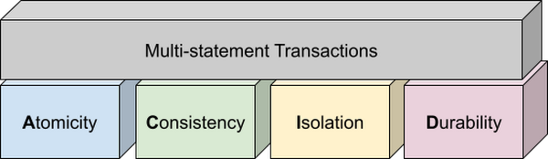
Transactions are known for their atomicity, consistency, isolation, and durability (ACID) properties. Atomicity indicates that all data changes (including metadata changes) are applied or reverted in a single operation, e.g. when a set of rows are added to a table with enrichment and the corresponding set of rows deleted, both operations happen together. Consistency refers to the consistency of data before and after the transaction has completed. When data is added to or updated in a table, the changes to data in tables are consistent with the constraints specified on the table or its columns, e.g. ensuring that the NOT NULL constraint is complied with when data gets added or modified in a table. Isolation indicates that multiple transactions can make changes to the table concurrently as long as the changes don’t conflict with each other, e.g. two transactions loading data into tables from different business units can proceed concurrently. Durability is the last and possibly the most important property of transactions which guarantees that in the event of a failure (after completing the transaction), all the changes committed by the transaction are saved for future transactions or queries.
Isolation level
All transactions in BigQuery including multi-statement transactions support snapshot isolation. At this isolation level, all statements in a transaction see a consistent snapshot of the database, as of the start of the transaction. BigQuery achieves this due to its multi-version property where it maintains the history of mutations to the database for a certain period. Transactions do not see any changes, committed or uncommitted, from other concurrent transactions while the transaction is in progress. BigQuery supports read-your-own-writes, where statements in a transaction can see all the changes applied by prior statements in the same transaction.
Example
Let’s run through an example to demonstrate how BigQuery supports the concept of multi-statement transactions with multiple sets of changes across multiple tables in one operation. In this example, we will set up this demo by creating 10 tables each with 100 partitions
Language: SQL
DECLARE num_tables DEFAULT 10;DECLARE x INT64 DEFAULT 0;# replace "demo" with your preferred dataset nameDECLARE ds STRING default "`00jathreya`";DECLARE prefix STRING DEFAULT "mst_demo";DECLARE table_name STRING;DECLARE pre_table_name STRING;/*Sets up 10 tables, with schema (partition_id:integer,value:timestamp).Each table has 100 partitions, with partition key 0, 10, 20, ..., 990.*/SET x = 0;WHILE x < num_tables DOSET table_name = format("%s.%s_%d", ds, prefix, x);EXECUTE IMMEDIATE format("""DROP TABLE IF EXISTS %s""", table_name);EXECUTE IMMEDIATE format("""CREATE OR REPLACE TABLE %s (partition_id INT64, value TIMESTAMP)PARTITION BY RANGE_BUCKET(partition_id, GENERATE_ARRAY(0, 1000, 10))AS SELECT partition_id, CURRENT_TIMESTAMP() AS value FROM UNNEST(GENERATE_ARRAY(0, 990, 10)) AS partition_id""", table_name);SET x = x + 1;END WHILE;# Verify the partitioned tables created and the timestampexecute immediate format("""select table_schema, table_name, count(partition_id), sum(total_rows), max(last_modified_time) from %s.INFORMATION_SCHEMA.PARTITIONSwhere starts_with(table_name,'%s')group by table_schema, table_name""", ds, prefix);# Verify data in table 9 based on the timestampEXECUTE IMMEDIATE format("""SELECT * FROM %s ORDER BY partition_id""", table_name);
Next, we will show how the new COMMIT and ROLLBACK commands in BigQuery allow you to save or reverse the changes in a transaction spanning multiple tables.
Language: SQL
DECLARE num_tables DEFAULT 10;DECLARE x INT64 DEFAULT 0;# Replace `mydataset` with your preferred dataset nameDECLARE ds STRING DEFAULT "`mydataset`";DECLARE prefix STRING DEFAULT "mst_demo";DECLARE table_name STRING;DECLARE pre_table_name STRING;/*Steps of the transaction:1. For table 0, updates the timestamp to CURRENT_TIMESTAMP.2. FOR table 1 to 9, merge table x using data from table x-1. All MERGE shouldsee the updated data in table x-1, so as a result the change in table 0 should bepropagated all the way to table 9.3. A total of 1000 partition changes on 10 tables.*/BEGIN TRANSACTION;SET x = 0;WHILE x < num_tables DOSET table_name = format("%s.%s_%d", ds, prefix, x);IF x = 0 THENEXECUTE IMMEDIATE format("""UPDATE %s SET value = CURRENT_TIMESTAMP WHERE true""", table_name);ELSESET pre_table_name = format("%s.%s_%d", ds, prefix, x-1);EXECUTE IMMEDIATE format("""MERGE %s t2 USING %s t1 ON t2.partition_id = t1.partition_idWHEN MATCHED THEN UPDATE SET value = t1.value""", table_name, pre_table_name);END IF;SET x = x + 1;END WHILE;# Verify data in table 9 inside transaction shows recently updated dataSET table_name = format("%s.%s_%d", ds, prefix, num_tables-1);EXECUTE IMMEDIATE format("""SELECT * FROM %s ORDER BY partition_id""", table_name);IF x = 9 THENCOMMIT TRANSACTION;ELSEROLLBACK TRANSACTION;END IF;# Verify data in table 9 outside transaction shows timestamp of original dataEXECUTE IMMEDIATE format("""SELECT * FROM %s ORDER BY partition_id""", table_name);
Monitoring and Management
Unlike single-statement transactions which map to a single DML command, multi-statement transactions are complex spanning multiple DML operations across multiple tables. To monitor these complex jobs, the BigQuery JOBS INFORMATION_SCHEMA views have been expanded to add a new column, TRANSACTION_ID, which contains a unique identifier for each transaction in BigQuery. You can query transactions that are in progress or the ones that have completed by querying these views.
Language: SQL
#Returns the list of transactions running under a parent job ID .;SELECTDISTINCT transaction_idFROM `region-us`.INFORMATION_SCHEMA.JOBS_BY_PROJECTWHERE parent_job_id = "job_id" AND state = "RUNNING";# Returns the active transactions and parent job id that are running and affect a named table.;WITHrunning_transactions AS (SELECT DISTINCT transaction_idFROM `region-us`.INFORMATION_SCHEMA.JOBS_BY_PROJECTWHERE state = "RUNNING")SELECTtransaction_id, parent_job_id, queryFROM `region-us`.INFORMATION_SCHEMA.JOBS_BY_PROJECT, running_transactionsWHERE destination_table = "mytable"AND transaction_id = running_transactions.transaction_id;# Returns all successfully committed transactionsSELECTtransaction_id, parent_job_id, queryFROM `region-us`.INFORMATION_SCHEMA.JOBS_BY_PROJECTWHERE statement_type = "COMMIT_TRANSACTION" AND error_result IS NULL;# Returns all rolled back transactionsSELECTtransaction_id, parent_job_id, queryFROM `region-us`.INFORMATION_SCHEMA.JOBS_BY_PROJECTWHERE statement_type = "ROLLBACK_TRANSACTION" AND error_result IS NULL;
To terminate a transaction, you will need to terminate the parent job under which the transaction is running by passing the parent job ID of the script containing the transaction to the BQ.JOBS.CANCEL system procedure.
Conclusion
As enterprises accelerate towards more real time insight-driven decisions, multi-statement transactions are a key enabler towards bringing transaction data into analytical data warehouses, such as BigQuery. With strong ACID properties, full transaction support for commit and rollback, and rich monitoring and management APIs built on proven transaction processing backbone, we are very pleased to help our BigQuery customers unlock the value of transactions through these new capabilities.
Soundtrack Your Brand: Delivering Sound That Stands Out From the Crowd with BigQuery

2837
Of your peers have already read this article.
6:00 Minutes
The most insightful time you'll spend today!
Editor’s note: Soundtrack Your Brand is an award-winning streaming service with the world’s largest licensed music catalog built just for businesses, backed by Spotify. Today, we hear how BigQuery has been a foundational component in helping them transform big data into music.
Soundtrack Your Brand is a music company at its heart, but big data is our soul. Playing the right music at the right time has a huge influence on the emotions a brand inspires, the overall customer experience, and sales. We have a catalog of over 58 million songs and their associated metadata from our music providers and a vast amount of user data that helps us deliver personalized recommendations, curate playlists and stations, and even generate listening schedules. As an example, through our Schedules feature our customers can set up what to play during the week. Taking that one step further, we provide suggestions on what to use in different time slots and recommend entire schedules.
Using BigQuery, we built a data lake to empower our employees to access all this content and metadata in a structured way. Ensuring that our data is easily discoverable and accessible allows us to build any type of analytics or machine learning (ML) use case and run queries reliably and consistently across the complete data set. Today, our users are benefiting from this advanced analytics through the personalized recommendations we offer across our core features: Home, Search, Playlists, Stations, and Schedules.
Fine-tuning developer productivity
The biggest business value that comes from BigQuery is how much it speeds up our development capabilities and allows us to ship features faster. In the past 3 years, we have built more than 150 pipelines and more than 30 new APIs within our ML and data teams that total about 10 people. That is an impressive rate of a new pipeline every week and a new API every month. With everything in BigQuery, it’s easy to simply write SQL and have it be orchestrated within a CI/CD toolchain to automate our data processing pipelines. An in-house tool built as a github template, in many ways very similar to Dataform, helps us build very complex ETL processes in minutes, significantly reducing the time spent on data wrangling.
BigQuery acts as a cornerstone for our entire data ecosystem, a place to anchor all our data and be our single source of truth. This single source of truth has expanded the limits of what we can do with our data. Most of our pipelines start from a data lake, or end at a data lake, increasing re-usability of data and collaboration. For example, one of our interns built an entire churn prediction pipeline in a couple of days on top of existing tables that are produced daily. Nearly a year later, this pipeline is still running without failure largely due to its simplicity. The pipeline is BigQuery queries chained together into a BigQuery ML model running on a schedule with Kubeflow Pipelines.
Once we made BigQuery the anchor for our data operations, we discovered we could apply it to use cases that you might not expect, such as maintaining our configurations or supporting our content management system. For instance, we created a Google Sheet where our music experts are able to correct genre classification mistakes for songs by simply adding a row to a Google Sheet. Instead of hours or days to create a bespoke tool, we were able to set everything up in a few minutes.
BigQuery’s ability to consume Excel spreadsheets allows business users who play key roles in improving our recommendations engine and curating our music, such as our content managers and DJs, to contribute to the data pipeline.
Another example is our use of BigQuery as an index for some of our large Cloud Storage buckets. By using cloud functions to subscribe to read/write events for a bucket, and writing those events to partitioned tables, our pipelines can easily and in a natural way quickly search and access files, such as downloading and processing the audio of new track releases. We also make use of Log Events when a table is added to a dataset to trigger pipelines that process data on demand, such as JSON/CSV files from some of our data providers that are newly imported into BQ. Being the place for all file integration and processing, BQ allows new data to be quickly available to our entire data ecosystem in a timely and cost effective manner while allowing for data retention, ETL, ACL and easy introspection.
BigQuery makes everything simple. We can make a quick partitioned table and run queries that use thousands of CPU hours to sift through a massive volume of data in seconds — and only pay a few dollars for the service. The result? Very quick, cost-effective ETL pipelines.
In addition, centralizing all of our data in BigQuery makes it possible to easily establish connections between pipelines providing developers with a clear understanding of what specific type of data a pipeline will produce. If a developer wants a different outcome, she can copy the github template and change some settings to create a new, independent pipeline.
Another benefit is that developers don’t have to coordinate schedules or sync with each other’s pipelines: they just need to know that a table that is updated daily exists and can be relied on as a data source for an application. Each developer can progress their work independently without worrying about interfering with other developers’ use of the platform.
Making iteration our forte
Out of the box, BigQuery met and exceeded our performance expectations, but ML performance was the area that really took us by surprise. Suddenly, we found ourselves going through millions of rows in a few seconds, where the previous method might have taken an hour. This performance boost ultimately led to us improving our artist clustering workload from more than 24 hours on a job running 100 CPU workers to 10 minutes on a BigQuery pipeline running inference queries in a loop until convergence. This more than 140x performance improvement also came at 3% of the cost.
Currently we have more than 100 Neural Network ML models being trained and run regularly in batch in BQML. This setup has become our favorite method for both fast prototyping and creating production ready models. Not only is it fast and easy to hypertune in BQML, but our benchmarks show comparable performance metrics to using our own Tensorflow code. We now use Tensorflow sparingly. Differences in input data can have an even greater impact on the experience of the end user than individual tweaks to the models.
BigQuery’s performance makes it easy to iterate with the domain experts who help shape our recommendations engine or who are concerned about churn, as we are able to show them the outcome on our recommendations from changes to input data in real-time. One of our favorite things to do is to build a Data Studio report that has the ML.predict query as part of its data source query. This report shows examples of good/bad predictions in the report along with bias/variance summaries and a series of drop-downs, thresholds and toggles to control the input features and the output threshold. We give that report to our team of domain experts to help manually tune the models, putting the model tuning right in the hands of the domain experts. Having humans in the loop has become trivial for our team. In addition to fast iteration, the BigQuery ML approach is also very low maintenance. You don’t need to write a lot of Python or Scala code or maintain and update multiple frameworks—everything can be written as SQL queries run against the data store.
Helping brands to beat the band—and the competition
BigQuery has allowed us to establish a single source of truth for our company that our developers and domain experts can build on to create new and innovative applications that help our customers find the sound that fits their brand.
Instead of cobbling together data from arbitrary sources, our developers now always start with a data set from BigQuery and build forward. This guarantees the stability of our data pipeline and makes it possible to build outward into new applications with confidence. Moreover, the performance of BigQuery means domain experts can interact with the analytics and applications that developers create more easily and see the results of their recommended improvements to ML models or data inputs quickly. This rapid iteration drives better business results, keeps our developers and domain experts aligned, and ensures Soundtrack Your Brand keeps delivering sound that stands out from the crowd.
5 Best Practices for Cloud Cost Optimization

5795
Of your peers have already read this article.
3:30 Minutes
The most insightful time you'll spend today!
When customers migrate to Google Cloud Platform (GCP), their first step is often to adopt Compute Engine, which makes it easy to procure and set up virtual machines (VMs) in the cloud that provide large amounts of computing power. Launched in 2012, Compute Engine offers multiple machine types, many innovative features, and is available in 20 regions and 61 zones!
Compute Engine’s predefined and custom machine types make it easy to choose VMs closest to your on-premises infrastructure, accelerating the workload migration process cost effectively. Cloud allows you the pricing advantage of ‘pay as you go’ and also provides significant savings as you use more compute with Sustained Use Discounts.
As Technical Account Managers, we work with large enterprise customers to analyze their monthly spend and recommend optimization opportunities. In this blog, we will share the top recommendations that we’ve developed based on our collective experience working with GCP customers.
Getting ready to save
Before you get started, be sure to familiarize yourself with the VM instance pricing page—required reading for anyone who needs to understand the Compute Engine billing model and resource-based pricing. In addition to those topics, you’ll also find information about the various Compute Engine machine types, committed use discounts and how to view your usage, among other things.
Another important step to gain visibility into your Compute Engine cost is using Billing reports in the Google Cloud Console and customizing your views based on filtering and grouping by projects, labels and more. From there you can export Compute Engine usage details to BigQuery for more granular analysis. This allows you to query the datastore to understand your project’s vCPU usage trends and how many vCPUs can be reclaimed. If you have defined thresholds for the number of cores per project, usage trends can help you spot anomalies and take proactive actions. These actions could be rightsizing the VMs or reclaiming idle VMs.
Now, with these things under your belt, let’s go over the five ways you can optimize your Compute Engine resources that we believe will give you the most immediate benefit.
1. Apply Compute Engine rightsizing recommendations
Compute Engine’s rightsizing recommendations feature provides machine type recommendations that are generated automatically based on system metrics gathered by Stackdriver Monitoring over the past eight days. Use these recommendations to resize your instance’s machine type to more efficiently use the instance’s resources. It also recommends custom machine types when appropropriate. Compute Engine makes viewing, resizing and other actions easier right from the Cloud Console as shown below.
Recently, we expanded Compute Engine rightsizing capabilities from just individual instances to managed instance groups as well. Check out the documentation for more details.
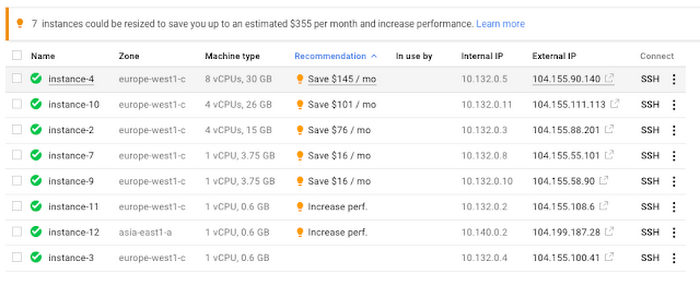
For more precise recommendations, you can install the Stackdriver Monitoring agent which collects additional disk, CPU, network, and process metrics from your VM instances to better estimate your resource requirements. You can also leverage the Recommender API for managing recommendations at scale.
2. Purchase Commitments
Our customers have diverse workloads running on Google Cloud with differing availability requirements. Many customers follow a 70/30 rule when it comes to managing their VM fleet—they have constant year-round usage of ~70%, and a seasonal burst of ~30% during holidays or special events.
If this sounds like you, you are probably provisioning resources for peak capacity. However, after migrating to Google Cloud, you can baseline your usage and take advantage of deeper discounts for Compute workloads. Committed Use Discounts are ideal if you have a predictable steady-state workload as you can purchase a one or three year commitment in exchange for a substantial discount on your VM usage.
We recently released a Committed Use Discount analysis report in the Cloud Console that helps you understand and analyze the effectiveness of the commitments you’ve purchased. In addition to this, large enterprise customers can work with their Technical Account Managers who can help manage their commitment purchases and work proactively with them to increase Committed Use Discount coverage and utilization to maximize their savings.
3. Automate cost optimizations
The best way to make sure that your team is always following cost-optimization best practices is to automate them, reducing manual intervention.
Automation is greatly simplified using a label—a key-value pair applied to various Google Cloud services. For example, you could label instances that only developers use during business hours with “env: development.” You could then use Cloud Scheduler to schedule a serverless Cloud Function to shut them down over the weekend or after business hours and then restart them when needed. Here is an architecture diagram and code samples that you can use to do this yourself.
Using Cloud Functions to automate the cleanup of other Compute Engine resources can also save you a lot of time and money. For example, customers often forget about unattached (orphaned) persistent disk, or unused IP addresses. These accrue costs, even if they are not attached to a virtual machine instance. VMs with the “deletion rule” option set to “keep disk” retain persistent disks even after the VM is deleted. That’s great if you need to save the data on that disk for a later time, but those orphaned persistent disks can add up quickly and are often forgotten! There is a Google Cloud Solutions article that describes the architecture and sample code for using Cloud Functions, Cloud Scheduler, and Stackdriver to automatically look for these orphaned disks, take a snapshot of them, and remove them. This solution can be used as a blueprint for other cost automations such as cleaning up unused IP addresses, or stopping idle VMs.
4. Use preemptible VMs
If you have workloads that are fault tolerant, like HPC, big data, media transcoding, CI/CD pipelines or stateless web applications, using preemptible VMs to batch-process them can provide massive cost savings. In fact, customer Descartes Labs reduced their analysis costs by more than 70% by using preemptible VMs to process satellite imagery and help businesses and governments predict global food supplies.
Preemptible VMs are short lived— they can only run a maximum of 24 hours, and they may be shut down before the 24 hour mark as well. A 30-second preemption notice is sent to the instance when a VM needs to be reclaimed, and you can use a shutdown script to clean up in that 30-second period. Be sure to fully review the full list of stipulations when considering preemptible VMs for your workload. All machine types are available as preemptible VMs, and you can launch one simply by adding “-preemptible” to the gcloud command line or selecting the option from the Cloud Console.
Using preemptible VMs in your architecture is a great way to scale compute at a discounted rate, but you need to be sure that the workload can handle the potential interruptions if the VM needs to be reclaimed. One way to handle this is to ensure your application is checkpointing as it processes data, i.e., that it’s writing to storage outside the VM itself, like Google Cloud Storage or a database. As an example, we have sample code for using a shutdown script to write a checkpoint file into a Cloud Storage bucket. For web applications behind a load balancer, consider using the 30-second preemption notice to drain connections to that VM so the traffic can be shifted to another VM. Some customers also choose to automate the shutdown of preemptible VMs on a rolling basis before the 24-hour period is over, to avoid having multiple VMs shut down at the same time if they were launched together.
5. Try autoscaling
Another great way to save on costs is to run only as much capacity as you need, when you need it. As we mentioned earlier, typically around 70% of capacity is needed for steady-state usage, but when you need extra capacity, it’s critical to have it available. In an on-prem environment, you need to purchase that extra capacity ahead of time. In the cloud, you can leverage autoscaling to automatically flex to increased capacity only when you need it.
Compute Engine managed instance groups are what give you this autoscaling capability in Google Cloud. You can scale up gracefully to handle an increase in traffic, and then automatically scale down again when the need for instances is lowered (downscaling). You can scale based on CPU utilization, HTTP load balancing capacity, or Stackdriver Monitoring metrics. This gives you the flexibility to scale based on what matters most to your application.
High costs do not compute
As we’ve shown above, there are many ways to optimize your Compute Engine costs. Monitoring your environment and understanding your usage patterns is key to understanding the best options to start with, taking the time to model your baseline costs up front. Then, there are a wide variety of strategies to implement depending on your workload and current operating model.
For more on cost management, check out our cost management video playlist. And for more tips and tricks on saving money on other GCP services, check out our blog posts on Cloud Storage, Networking and BigQuery cost optimization strategies. We have additional blog posts coming soon, so stay tuned!
4024
Of your peers have already watched this video.
54:30 Minutes
The most insightful time you'll spend today!
Quick Tips to Get the Most Out of Cloud Spanner
Today, IT Admins and DBAs are inundated with thankless tasks. But they no longer have to deal with that. With Cloud Spanner, they can focus on value-add and innovation instead of maintenance. Creating or scaling a globally replicated database for mission-critical apps now takes a handful of clicks.
Industry-leading high-availability and Google-grade security as defaults, not expensive add-ons, help ensure your apps stay online and more secure.
Cloud Spanner is a powerful product, but many users do not maximize its benefits.
It is the first scalable, enterprise-grade, globally-distributed, and strongly consistent database service built for the cloud specifically to combine the benefits of relational database structure with a non-relational horizontal scale.
This combination delivers high-performance transactions and strong consistency across rows, regions, and continents with an industry-leading 99.999% availability SLA, no planned downtime, and enterprise-grade security. Cloud Spanner revolutionizes database administration and management and makes application development more efficient.
This video highlights best practices, strategies for optimizing applications and workloads, and ways to improve performance and scalability. This live demos shows real-time speed-ups of transactions, queries, and overall performance.
Additionally, this talk explores techniques for monitoring Cloud Spanner to identify performance bottlenecks. Watch now to learn more.
AWS to Google Cloud Translator: Which AWS Database Service Is Equal to Google Cloud Database?

6314
Of your peers have already read this article.
2:30 Minutes
The most insightful time you'll spend today!
There are multiple reasons a growing number of database administrators, enterprise architects, application developers and other technology practitioners are moving to Google Cloud’s various database services.
Some are being driven by missing features in offering from other providers such as AWS. In Gartner’s Magic Quadrant for Operational Database Management Systems, the research and advisory firm points out that, “AWS’s surveyed reference customers scored its overall product capabilities one standard deviation (STD) below the mean. Their responses identified missing features such as multiregion writes and autosharding.”
Others are moving to database services on Google Cloud Platform driven by a few benefits. According to Gartner, “Reference customers repeatedly commented on Google’s ease of use and implementation, reliability and integration (with other services and other systems). Reference customers scored Google a full STD above the mean for satisfaction with GCP’s pricing; it received the second-highest satisfaction score of any vendor in this Magic Quadrant.
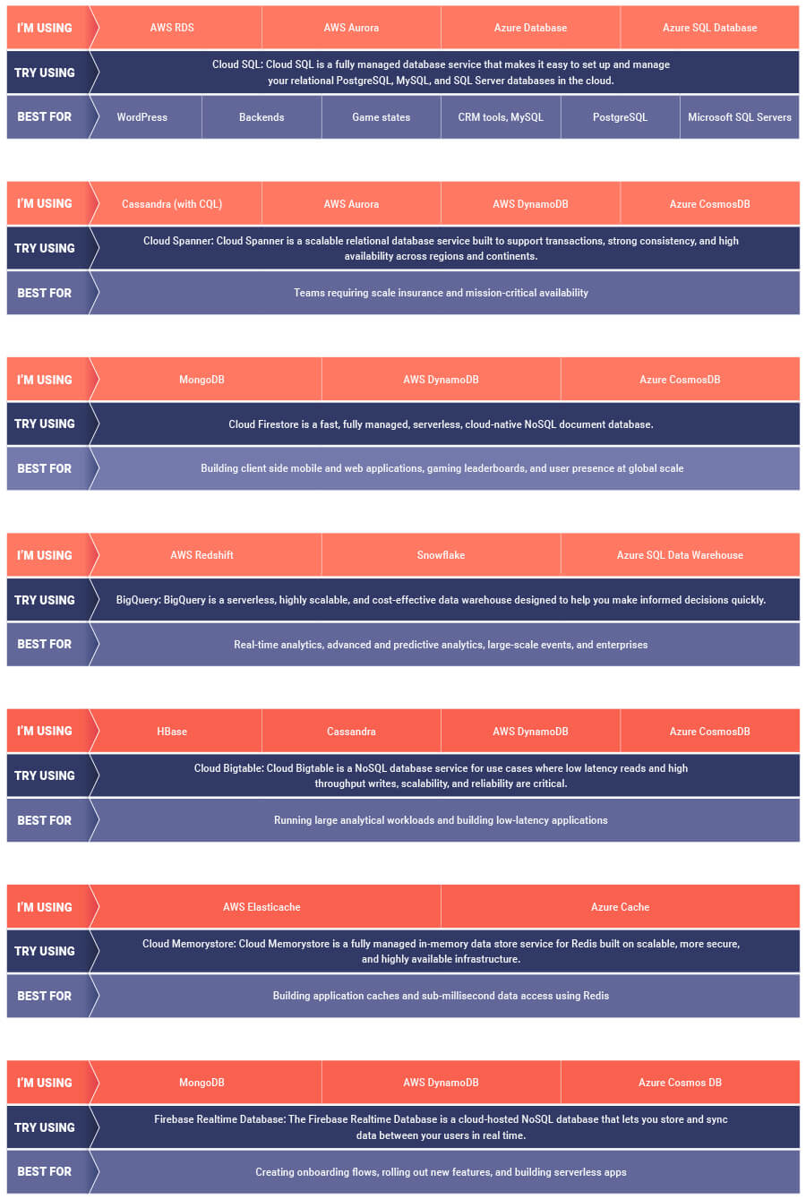
If you are looking to leverage the power of Google Cloud database offerings—but were unsure of which database services comes closest to the service you are currently using, here’s a handy map to find your way.
Case Study: When Database Choice Powers New Revenue-driving Product Features

4166
Of your peers have already read this article.
4:30 Minutes
The most insightful time you'll spend today!
Editor’s note: Streak makes a CRM add-on for Gmail, and recently adopted Cloud Spanner to take advantage of its scalability and SQL capabilities to implement a graph data model. Read on to learn about their decision, what they love about the system, and the ways in which it still needs work.]
Streak is a customer relationship management (CRM) tool built directly into Gmail. It is used for sales, marketing, hiring, and just about anything else you can think of.
We built it because out of the box, email is actually a really crummy team sharing system. By adding a layer of organization on top of email, Streak lets you add email threads directly into its spreadsheet view, making it useful as a workflow tool with capabilities including task creation, email template management, and easy data entry.
Streak has been integrated with G Suite (originally Google Apps For Your Domain) since its inception so when choosing a cloud, it made sense to colocate our server stack with Google Cloud.
Likewise, Streak was on Google App Engine from the start, and we slowly added other GCP services as the offerings improved or as our use cases became more complex.
In addition to App Engine, we use Google Kubernetes Engine to run a bunch of our compute workload, including both application servers and our offline processes like indexers and task queue consumers.
We use Cloud Dataflow for both streaming event processing and logs ETL, and BigQuery for all of our analytics queries. We use Cloud Pub/Sub for interacting with the Gmail watch API, as well as Stackdriver (logging, tracing, monitoring, errors) and OpenCensus to dig into any operational issues as they arise.
Then, on the database front, we recently started using Cloud Spanner, Google Cloud’s scalable relational database service. Before that, we stored most of our business data in Cloud Datastore, Google Cloud’s NoSQL document database.
Partially, that was historical, since Cloud Datastore was GCP’s only managed database when we wrote the Streak backend. And we’ve been very happy with how easy Cloud Datastore is to maintain. Between Google App Engine and Cloud Datastore, we’ve never had to have an explicit infrastructure on-call rotation.
But as more users rely on Streak to collaborate with larger and larger teams, we were feeling the pain of not having a fully relational database. We found ourselves having to manually join data in our application, which increased application latency and increased the time developers spent coding workarounds and debugging that complexity.
We found we needed two things out of our database: a scalable relational store and a graph store that could power next-gen Streak features. At the same time, we wanted a single database that could handle both use cases and wouldn’t increase our operational burden. This meant finding a managed service to give us more query flexibility, so we decided to give Cloud Spanner a try.
Of course, we didn’t want to migrate our existing stack to a new data platform without first testing it out (never a smart strategy). But since most of our existing data model required transactional updates with other entities, pulling out a single entity to test was challenging. We did have a feature in our pipeline that necessitated a graph data store and that was removed from our other data: our email metadata indexing system.
How your client software handles email metadata indexing can make or break the useability of a system. Think about how many times somebody forgets to reply-all or that you receive a forwarded thread with thirty emails in reverse-chronological order. Within our own inboxes, we rely on Gmail’s UI to nicely organize email threads, but that organization breaks down when working with a team or across organizational boundaries.
We decided to fix that in the Streak product by organizing metadata (i.e., headers but not message content) from users’ email by using Cloud Spanner as a graph database. Using a graph database lets us answer questions like “What are all the emails on this thread in the inboxes of everybody on my team?” and “Who on my team has previously talked with the organization that this prospect works at?”
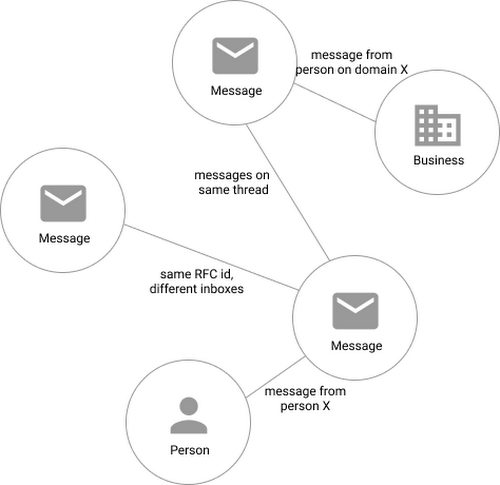
In our model, the nodes of the graph are either an email message, a person (email address) or a company (a domain). Then we have four different types of “edges”— properties by which nodes in a graph connect to one another:
- Message to message (thread): messages that are on the same thread have an edge between them. The reason we do this is because we want to show users a list of threads to answer their questions, not messages, so we need to be able to get the spanning set of messages.
- Message to message (same RFC id): A core value proposition of Streak is being able to see the “unified” version of a thread that shows each person on a team’s version of the email thread. To make sure we are getting each user’s version of a thread when we issue a query, there needs to be an edge between a message in the queryer’s inbox and the same message in their team’s inbox. In case you’re curious, Streak uses the RFC message id to determine that two messages across inboxes are actually the same.
- Email address to message: a message has an edge to an email address if it was either the from, to, cc, or bcc on the message. This edge is crucial for queries that start with: “Show me all threads between this person and our team.”
Domain to message: a message has an edge to a domain if the domain is present in any of the from, to, cc, or bcc addresses on the message. This edge is similarly used for queries that start with “Show me all threads between this company and our team.”
Using Cloud Spanner’s distributed SQL capabilities and scalability to build a graph database also let us answer the important follow-up question: “Which threads have I been granted permission to view?” And while a lot of these questions could be answered per-user by a traditional relational database, scale limitations have to be taken into consideration, especially as we plan for 10x or more data volume growth as both our user base grows and as their inboxes accumulate more emails. A graph database model is simply a better fit for Streak’s collaboration model with many-to-many mappings between users and teams, and will allow us to query the data in any number of configurations, without worrying about scale limitations or having to manually shard a relational database. Cloud Spanner gives us queryability and scalability.
Taking the Cloud Spanner plunge
With so many advantages to it, we went ahead and began building out our metadata system with Cloud Spanner as a back-end.
Adopting Cloud Spanner has been great. Here are some of the high points:
- The fast distributed queries and transactions are absolutely real. We have global indexes across our entire dataset and we haven’t had to spend very much time at all thinking about co-locating data. In particular, we only use interleaved tables for values that would be repeated fields in Cloud Datastore, and that hasn’t been a problem for us yet.
- We haven’t had any reliability problems whatsoever, despite averaging 20K writes/sec in steady state.
- Once we optimized our queries on realistic data, Cloud Spanner scaled up in a surprisingly predictable way. You need to run queries after you’ve populated data, do the explain to figure out how the query planner is executing the query, and add indexes/modify queries to make sure they’re performant.
- Compared to the hoops some traditional relational databases make you jump through, Cloud Spanner’s online schema changes and index builds are magical. There is no downtime for these operations.
Overall, the experience has been encouraging, and we’re planning to move 20 TB of existing data in Cloud Datastore to Cloud Spanner as well. We built out an ORM library for Java on top of Cloud Spanner called Ratchet and are testing a framework for dual-writing entities to both Cloud Datastore and Cloud Spanner to support the rest of the migration. We now store about 40 TB of email metadata in Cloud Spanner, which makes us a large user of Cloud Spanner.
In short, if you’re starting to outgrow your NoSQL database, and want to move to a managed SQL database, give Cloud Spanner a try. You definitely want to model out your costs and try out a proof of concept, both to see how it works on your workload and to get familiar with the quirks of the system. But you don’t need to spend much time worrying about the reliability of the product: it’s there.
More Relevant Stories for Your Company

Transforming Software Development Education with CourseMatix
As the world increasingly relies on software, businesses have struggled to find enough developer talent to build and maintain their applications. IDC estimates the global shortage of software developers reached 1.4 million in 2021 and expects that number to balloon to 4 million by 2025. Higher education is a great starting

Boost Database Performance with AlloyDB Index Advisor: The Ultimate Optimization Tool
Intro One of the time consuming tasks for DBAs is to maximize query performance. To optimize slow-running queries, they often have to do detailed analysis, understand optimizer plans, and go through a lot of trial and error before getting to the best set of indexes that help with improved query

AgroStar: Small farms in India getting big help from the cloud
AgroStar has launched a cloud-based mobile app that is helping to boost crop yields and encourage best practices for small farmers in India. Launched as an on-premises ecommerce platform selling farm tools in 2008, the firm turned to Google Cloud Platform (GCP) to expand its offering. It now uses cloud-based analytics and is

BigQuery Reference Guide: Understanding Tables within and Routine for Data Transformation
Last week in our BigQuery Reference Guide series, we spoke about the BigQuery resource hierarchy - specifically digging into project and dataset structures. This week, we’re going one level deeper and talking through some of the resources within datasets. In this post, we’ll talk through the different types of tables
