There are multiple reasons a growing number of database administrators, enterprise architects, application developers and other technology practitioners are moving to Google Cloud’s various database services.

Some are being driven by missing features in offering from other providers such as AWS. In Gartner’s Magic Quadrant for Operational Database Management Systems, the research and advisory firm points out that, “AWS’s surveyed reference customers scored its overall product capabilities one standard deviation (STD) below the mean. Their responses identified missing features such as multiregion writes and autosharding.”

Others are moving to database services on Google Cloud Platform driven by a few benefits. According to Gartner, “Reference customers repeatedly commented on Google’s ease of use and implementation, reliability and integration (with other services and other systems). Reference customers scored Google a full STD above the mean for satisfaction with GCP’s pricing; it received the second-highest satisfaction score of any vendor in this Magic Quadrant.

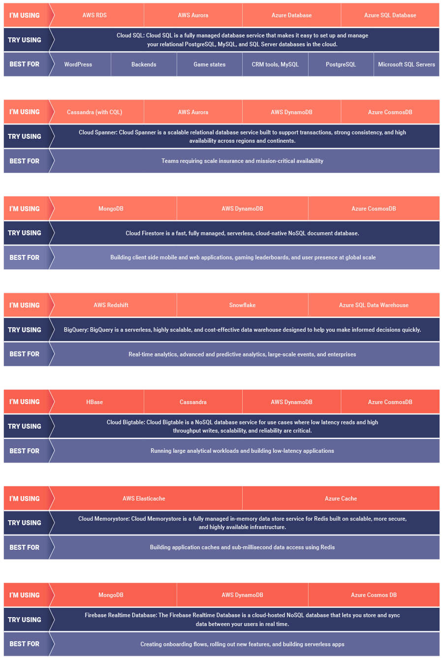
If you are looking to leverage the power of Google Cloud database offerings—but were unsure of which database services comes closest to the service you are currently using, here’s a handy map to find your way.

Editor’s note: Streak makes a CRM add-on for Gmail, and recently adopted Cloud Spanner to take advantage of its scalability and SQL capabilities to implement a graph data model. Read on to learn about their decision, what they love about the system, and the ways in which it still needs work.]  

Streak is a customer relationship management (CRM) tool built directly into Gmail. It is used for sales, marketing, hiring, and just about anything else you can think of.

We built it because out of the box, email is actually a really crummy team sharing system. By adding a layer of organization on top of email, Streak lets you add email threads directly into its spreadsheet view, making it useful as a workflow tool with capabilities including task creation, email template management, and easy data entry.

Streak has been integrated with G Suite (originally Google Apps For Your Domain) since its inception so when choosing a cloud, it made sense to colocate our server stack with Google Cloud.

Likewise, Streak was on Google App Engine from the start, and we slowly added other GCP services as the offerings improved or as our use cases became more complex.

In addition to App Engine, we use Google Kubernetes Engine to run a bunch of our compute workload, including both application servers and our offline processes like indexers and task queue consumers.

We use Cloud Dataflow for both streaming event processing and logs ETL, and BigQuery for all of our analytics queries. We use Cloud Pub/Sub for interacting with the Gmail watch API, as well as Stackdriver (logging, tracing, monitoring, errors) and OpenCensus to dig into any operational issues as they arise.

Then, on the database front, we recently started using Cloud Spanner, Google Cloud’s scalable relational database service. Before that, we stored most of our business data in Cloud Datastore, Google Cloud’s NoSQL document database.

Partially, that was historical, since Cloud Datastore was GCP’s only managed database when we wrote the Streak backend. And we’ve been very happy with how easy Cloud Datastore is to maintain. Between Google App Engine and Cloud Datastore, we’ve never had to have an explicit infrastructure on-call rotation.

But as more users rely on Streak to collaborate with larger and larger teams, we were feeling the pain of not having a fully relational database. We found ourselves having to manually join data in our application, which increased application latency and increased the time developers spent coding workarounds and debugging that complexity.

We found we needed two things out of our database: a scalable relational store and a graph store that could power next-gen Streak features. At the same time, we wanted a single database that could handle both use cases and wouldn’t increase our operational burden. This meant finding a managed service to give us more query flexibility, so we decided to give Cloud Spanner a try.

Of course, we didn’t want to migrate our existing stack to a new data platform without first testing it out (never a smart strategy). But since most of our existing data model required transactional updates with other entities, pulling out a single entity to test was challenging. We did have a feature in our pipeline that necessitated a graph data store and that was removed from our other data: our email metadata indexing system.

How your client software handles email metadata indexing can make or break the useability of a system.  Think about how many times somebody forgets to reply-all or that you receive a forwarded thread with thirty emails in reverse-chronological order. Within our own inboxes, we rely on Gmail’s UI to nicely organize email threads, but that organization breaks down when working with a team or across organizational boundaries.

We decided to fix that in the Streak product by organizing metadata (i.e., headers but not message content) from users’ email by using Cloud Spanner as a graph database. Using a graph database lets us answer questions like “What are all the emails on this thread in the inboxes of everybody on my team?” and “Who on my team has previously talked with the organization that this prospect works at?”

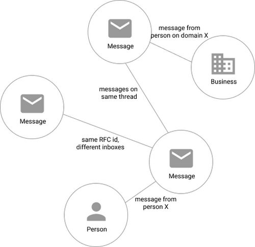
In our model, the nodes of the graph are either an email message, a person (email address) or a company (a domain). Then we have four different types of “edges”— properties by which nodes in a graph connect to one another:

1. Message to message (thread): messages that are on the same thread have an edge between them. The reason we do this is because we want to show users a list of threads to answer their questions, not messages, so we need to be able to get the spanning set of messages.
2. Message to message (same RFC id): A core value proposition of Streak is being able to see the “unified” version of a thread that shows each person on a team’s version of the email thread. To make sure we are getting each user’s version of a thread when we issue a query, there needs to be an edge between a message in the queryer’s inbox and the same message in their team’s inbox. In case you’re curious, Streak uses the RFC message id to determine that two messages across inboxes are actually the same.
3. Email address to message: a message has an edge to an email address if it was either the from, to, cc, or bcc on the message. This edge is crucial for queries that start with: “Show me all threads between this person and our team.”

Domain to message: a message has an edge to a domain if the domain is present in any of the from, to, cc, or bcc addresses on the message. This edge is similarly used for queries that start with “Show me all threads between this company and our team.”

Using Cloud Spanner’s distributed SQL capabilities and scalability to build a graph database also let us answer the important follow-up question: “Which threads have I been granted permission to view?” And while a lot of these questions could be answered per-user by a traditional relational database, scale limitations have to be taken into consideration, especially as we plan for 10x or more data volume growth as both our user base grows and as their inboxes accumulate more emails. A graph database model is simply a better fit for Streak’s collaboration model with many-to-many mappings between users and teams, and will allow us to query the data in any number of configurations, without worrying about scale limitations or having to manually shard a relational database. Cloud Spanner gives us queryability and scalability.

Taking the Cloud Spanner plunge

With so many advantages to it, we went ahead and began building out our metadata system with Cloud Spanner as a back-end.

Adopting Cloud Spanner has been great. Here are some of the high points:

1. The fast distributed queries and transactions are absolutely real. We have global indexes across our entire dataset and we haven’t had to spend very much time at all thinking about co-locating data. In particular, we only use interleaved tables for values that would be repeated fields in Cloud Datastore, and that hasn’t been a problem for us yet.
2. We haven’t had any reliability problems whatsoever, despite averaging 20K writes/sec in steady state.
3. Once we optimized our queries on realistic data, Cloud Spanner scaled up in a surprisingly predictable way. You need to run queries after you’ve populated data, do the explain to figure out how the query planner is executing the query, and add indexes/modify queries to make sure they’re performant.
4. Compared to the hoops some traditional relational databases make you jump through, Cloud Spanner’s online schema changes and index builds are magical. There is no downtime for these operations.

Overall, the experience has been encouraging, and we’re planning to move 20 TB of existing data in Cloud Datastore to Cloud Spanner as well. We built out an ORM library for Java on top of Cloud Spanner called Ratchet and are testing a framework for dual-writing entities to both Cloud Datastore and Cloud Spanner to support the rest of the migration. We now store about 40 TB of email metadata in Cloud Spanner, which makes us a large user of Cloud Spanner.

In short, if you’re starting to outgrow your NoSQL database, and want to move to a managed SQL database, give Cloud Spanner a try. You definitely want to model out your costs and try out a proof of concept, both to see how it works on your workload and to get familiar with the quirks of the system. But you don’t need to spend much time worrying about the reliability of the product: it’s there.

With summer just around the corner, things are really heating up. But you’re in luck because this month BigQuery is supplying a cooler full of ice cold refreshments with this release of user-friendly SQL capabilities. 

We are pleased to announce three categories of BigQuery user-friendly SQL launches: Powerful Analytics Features, Flexible Schema Handling, and New Geospatial Tools.

Powerful Analytics Features

These powerful SQL analytics features provide greater flexibility to analysts for organizing, filtering, and rendering data in BigQuery than ever before. You can enable spreadsheet-like functionality on summarized data using PIVOT and UNPIVOT and filter irrelevant data in analytic functions using QUALIFY.

Through this section, we will become familiar with these new features through examples using the BigQuery Public dataset, usa_names.

PIVOT/UNPIVOT (Preview)

One of the most time-consuming tasks for data analytics practitioners is wrangling data into the right shape. SQL is great for wrangling data, but sometimes you want to reformat a table as you would in a spreadsheet, pivoting rows and columns interchangeably. To support this use case, we are pleased to introduce PIVOT and UNPIVOT operators in BigQuery. PIVOT creates columns from unique values in rows by aggregating values, and UNPIVOT reverses this action.The example below uses PIVOT on bigquery-public-data.usa_names.usa_1910_current to show the number of males and females born each year, representing each gender as a column. Then UNPIVOT reverses this action.

Language: SQL

  -- we start with SQL to create a simple table
-- we only include gender, year, and number. 
CREATE TABLE
  mydataset.sampletable1 AS (
  SELECT
    Gender,Year,SUM(Number) AS Number
  FROM
    `bigquery-public-data.usa_names.usa_1910_current`
  WHERE
    Year >= 2017
  GROUP BY
    Gender, Year);
-- The resulting table:
--+----------------------------------------+
--|   Gender   |    Year    |    Number    |
--+----------------------------------------+
--|      F     |    2019    |    1353716   |
--|      F     |    2017    |    1403989   |
--|      F     |    2018    |    1380382   |
--|      M     |    2018    |    1568678   |
--|      M     |    2019    |    1538056   |
--|      M     |    2017    |    1604609   |
--+----------------------------------------+
-- use PIVOT to create columns for “female” and “male” 
CREATE TABLE
  mydataset.Pivoted AS
SELECT
  year, male, female
FROM
  mydataset.sampletable1 
PIVOT( SUM(Number) FOR gender IN ('M' AS male,
  'F' AS female))
ORDER BY
  year;
-- The resulting pivoted table:
--+----------------------------------------+
--|    Year    |   female   |     male     |
--+----------------------------------------+
--|    2017    |   1403989   |    1604609  |
--|    2018    |   1380382   |    1568678  |
--|    2019    |   1353716   |    1538056  |
--+----------------------------------------+
-- UNPIVOT reverses the row/column rotation of PIVOT.
SELECT
  *
FROM
  mydataset.Pivoted 
UNPIVOT(number FOR gender IN (male AS 'M',
  female AS 'F'));

QUALIFY (Preview)

More advanced users of SQL know the power of analytic functions (aka window functions). These functions compute values over a group of rows, returning a single result for each row. For example, customers use analytic functions to compute a grand total, subtotal, moving average, rank, and more. With the announcement of support for QUALIFY, BigQuery users can now filter on the results of analytic functions by using the QUALIFY clause. 

QUALIFY belongs in the family of query clauses used for filtering along with WHERE and HAVING. The WHERE clause is used to filter individual rows in a query. The HAVING clause is used to filter aggregate rows in a result set after aggregate functions and GROUP BY clauses. The QUALIFY clause is used to filter results of analytic functions. 

To show the utility of QUALIFY, the example below uses QUALIFY to return the top 3 female names from each year in the last decade using from bigquery-public-data.usa_names.usa_1910_current. 

Language: SQL

  -- QUALIFY filters the result of the RANK function
SELECT
  name,year,SUM(number) AS total,
  RANK() OVER (PARTITION BY year 
  ORDER BY SUM(number) DESC) AS rank
FROM
  `bigquery-public-data.usa_names.usa_1910_current`
WHERE
  gender = 'F'
  AND YEAR >= 2010
GROUP BY 1,2 
QUALIFY RANK <= 3
ORDER BY 2,4;

Flexible Schema Handling

New SQL for administrators and data engineers enables table renaming for data pipeline processes, as well as flexible column management.

Table Rename (GA)

In data pipeline processes, tables are often created and then renamed so that they can make way for the next iteration of the pipeline run. To accomplish this, customers need a mechanism by which they can create a table and then subsequently rename it. Now if customers want to change this name using SQL, they can. Using the simple syntax that ALTER TABLE RENAME TO provides, customers will be able to rename a table after creation to clear the way for the next iteration of tables in the data pipeline.

Language: SQL

  -- create a sample table “tablename” in “mydataset”. 
-- You will rename this table.
CREATE OR REPLACE TABLE dataset.tablename(
    col1 STRING, 
    col2 NUMERIC);
-- if this table “tablename” becomes obsolete
-- perform Table Rename to “obsoletetable”
ALTER TABLE
  mydataset.name RENAME TO obsoletetable;

DROP NOT NULL constraints on a column (GA)

While BigQuery has historically provided many tools available in the UI, CLI and APIs, we know that many administrators prefer interfacing with the database using SQL. BigQuery recently released DDL statements which enable data administrators to provision and manage datasets and tables, greatly simplifying provisioning and management. Today, we continue the next addition in this line of releases by announcing ALTER COLUMN DROP NOT NULL constraint on a column:

• ALTER COLUMN DROP NOT NULL allows the administrator to remove the NOT NULL constraint from a column in BigQuery.

Language: SQL

  -- create a table to store credit card numbers
-- the business requires this field, so 
-- include a NOT NULL constraint 
CREATE TABLE
  mydataset.customers(credit_card_number STRING NOT NULL);
-- if needs of the business no longer require this field,
-- the customer can allow null entries in this column
-- by dropping the constraint
ALTER TABLE
  mydataset.customers 
ALTER COLUMN credit_card_number DROP NOT NULL;

CREATE VIEW with column list (GA)

Views are used ubiquitously by BigQuery customers to capture business logic. Oftentimes, BigQuery users have business requirements to assign aliases to columns in views. Now BigQuery supports doing so upon view creation in a column name list format with the release of CREATE VIEW with column list syntax.

Language: SQL

  -- aliases list1 and list2 can be assigned in a list format
CREATE VIEW
  myview (list1, list2) AS
SELECT
  column_1, column_2
FROM
  mydataset.exampletable

New Geospatial Tools

ST_POINTN, ST_STARTPOINT, and ST_ENDPOINT

Geospatial data is incredibly valuable to data analytics customers dealing with data from the physical world. BigQuery has very strong geospatial function support to help customers process marketing data, track storms, or manage self-driving cars. Particularly for analyzing vehicle or location tracking data, we’re thrilled to provide three new functions to allow users to easily extract or filter on key points:  

• ST_POINTN
• ST_STARTPOINT
• ST_ENDPOINT

For example, when working with vehicle histories,  ST_POINTN, ST_STARTPOINT, and ST_ENDPOINT allow users to extract elements such as the start and the end of a trip. For identifying origin-destination pairs these functions will make that task much easier.

Language: SQL

  -- pull the first, second, penultimate and final points 
-- from a linestring
WITH linestring as (
    SELECT ST_GeogFromText('linestring(1 1, 2 1, 3 2, 3 3)') g
)
SELECT
  ST_StartPoint(g) AS first, ST_EndPoint(g) AS last,
  ST_PointN(g,2) AS second, ST_PointN(g, -2) as second_to_last
FROM
  linestring
+--------------+--------------+--------------+----------------+
| first        | last         | second       | second_to_last |
+--------------+--------------+--------------+----------------+
| POINT(1 1)   | POINT(3 3)   | POINT(2 1)   | POINT(3 2)     |
+--------------+--------------+--------------+----------------+

As sure as a hot summer day pairs well with an ice-cold beverage, these new user-friendly SQL features in BigQuery pair well with your data analytics workflows. To learn more about BigQuery, visit our website, and get started immediately with the free BigQuery Sandbox.

Google Cloud allows you to move your PostgreSQL databases to Cloud SQL with Database Migration Service (DMS). DMS gives you the ability to replicate data continuously to the destination database, while the source is live in production, enabling you to migrate with minimum downtime.

However, terabyte-scale migrations can be complex. For instance, if your PostgreSQL database has Large Objects, then you will require some downtime to migrate them manually as that is a limitation of DMS. There are few more such limitations – check out known limitations of DMS. If not handled carefully, these steps can extend the downtime during cutover, lead to performance impact on the source instance, or even delay the project delivery date. All this may mean significant business impact.

Searce is a technology consulting company, specializing in modernizing application and database infrastructure by leveraging cloud, data and AI. We empower our clients to accelerate towards the future of their business. In our journey, we have helped dozens of clients migrate to Cloud SQL, and have found terabyte-scale migrations to be the toughest for the reasons mentioned earlier.

This blog centers around our work in supporting an enterprise client whose objective was to migrate dozens of terabyte scale, mission-critical PostgreSQL databases to Cloud SQL with minimum downtime. Their largest database was 20TB in size and all the databases had tables with large objects and some tables did not have primary keys. Note that DMS had a limitation of not supporting migration of tables without a primary key during the time of this project. In June 2022, DMS released an enhancement to support the migration of tables without a primary key.

In this blog, we share with you our learnings about how we simplified and optimized this migration, so that you can incorporate our best practices into your own migrations. We explore mechanisms to reduce the downtime required for operations not handled by DMS by ~98% with the use of automation scripts. We also explore database flags in PostgreSQL to optimize DMS performance and minimize the overall migration time by ~15%.

Optimize DMS performance with database flags

Once the customer made the decision to migrate PostgreSQL databases to Google Cloud SQL, we considered two key factors that would decide business impact – migration effort and migration time. To minimize effort for the migration of PostgreSQL databases, we leveraged Google Cloud’s DMS (Database Migration Service) as it is very easy to use and it does the heavy lifting by continuously replicating data from the source database to the destination Cloud SQL instance, while the source database is live in production.

How about migration time? For a terabyte-scale database, depending on the database structure, migration time can be considerably longer. Historically, we observed that DMS took around 3 hours to migrate a 1 TB database. In other cases, where the customer database structure was more complex, migration took longer. Thankfully, DMS takes care of this replication while the source database is live in production, so no downtime is required during this time. Nevertheless, our client would have to bear the cost of both the source and destination databases which for large databases, might be substantial. Meanwhile, if the database size increased, then replication could take even longer, increasing the risk of missing the customer’s maintenance window for the downtime incurred during cutover operations. Since the customer’s maintenance window was monthly, we would have to wait for 30 more days for the next maintenance window, requiring the customer to bear the cost of both the databases for another 30 days. Furthermore, from a risk management standpoint, the longer the migration timeframe, the greater the risk that something could go wrong. Hence, we started exploring options to reduce the migration time. Even the slightest reduction in migration time could significantly reduce the cost and risk.

We explored options around tuning PostgreSQL’s database flags on the source database. While DMS has its own set of prerequisite flags for the source instance and database, we also found that flags like shared_buffers, wal_buffers and maintenance_work_mem helped accelerate the replication process through DMS. These flags needed to be set to a specific value to get the maximum benefit out of each of them. Once set, their cumulative impact was a reduction in time for DMS to replicate a 1 TB database by 4 hours, that is, reduction of 3.5 days for a 20 TB database. Let’s dive into each of them.

Shared Buffers

PostgreSQL uses two buffers – its own internal buffer and the kernel buffered IO. In other words, that data is stored in memory twice. The internal buffer is called shared_buffers, and it determines the amount of memory used by the database for the operating system cache. By default this value is set conservatively low. However, increasing this value on the source database to fit our use case helped increase the performance of read heavy operations, which is exactly what DMS does once a job has been initialized.

After multiple iterations, we found that if the value was set to 55% of the database instance RAM, it boosted the replication performance (a read heavy operation) by a considerable amount and in turn reduced the time required to replicate the data.

WAL Buffers

PostgreSQL relies on Write-Ahead Logging (WAL) to ensure data integrity. WAL records are written to buffers and then flushed to disk. The flag wal_buffers, determines the amount of shared memory used for WAL data that has not yet been written to disk – records that are yet to be flushed. We found that increasing the value for wal_buffers from the default value of 16MB to about 3% of the database instance’s RAM significantly improved the write performance by writing fewer but larger files to the disk at each transaction commit.

Maintenance Work Mem

PostgreSQL maintenance operations, such as VACUUM, CREATE INDEX, and ALTER TABLE ADD FOREIGN KEY, consume their own specific memory. This memory is referred to as maintenance_work_mem. Unlike other operations, PostgreSQL maintenance operations can only be performed sequentially by the database. Setting a value significantly higher than the default value of 64 MB meant that no maintenance operation would block the DMS job. We found that maintenance_work_mem worked best at the value of 1 GB.

Resize source instance to avoid performance impact

Each of these three flags tune how PostgreSQL utilizes memory resources. Hence, it was imperative that before setting these flags, we needed to upsize the source database instance to accommodate them. Without upsizing the database instances, we could have caused application performance degradation, as more than half of the total database memory would be allocated to the processes managed by these flags.

We calculated the memory required by the flags mentioned above, and found that each flag needed to be set to a specific percentage of the source instance’s memory, irrespective of the existing values that might be set for the flags:

• shared_buffers: 55% of source instance’s memory
• wal_buffers: 3% of source instance’s memory
• maintenance_work_mem: 1 GB

We added the individual memory requirements by the flags, and found that 58% of the RAM at least will be taken up by these memory flags. For example, if a source instance used 100GB of memory, 58GB would be taken up by shared_buffers and wal_buffers, and an additional 1GB by maintenance_work_mem. As the original value of these flags was very low (~200MB), we upsized the RAM of the source database instance by 60% in order to ensure that the migration did not impact source performance on the application live in production.

Avoid connection error with WAL sender timeout flag

While using Google Cloud’s DMS, if the connection is terminated between DMS and the Cloud SQL instance during the ‘Full Dump in Progress’ phase of the DMS job, the DMS job fails and needs to be reinitiated. Encountering timeouts, especially while migrating a terabyte-scale database, would mean multiple days’ worth of migration being lost and a delay in the cutover plan. For example, if the connection of the DMS job for a 20TB database migration is lost after 10 days, the DMS job will have to be restarted from the beginning, leading to 10 days’ worth of migration effort being lost.

Adjusting the WAL sender timeout flag (wal_sender_timeout) helped us avoid terminating replication connections that were inactive for a long time during the full dump phase. The default value for this flag is 60 seconds. To avoid these connections from terminating, and to avoid such high impact failures, we set the value of this flag to 0 for the duration of database migration. This would avoid connections getting terminated and allowed for smoother replication through the DMS jobs.

Generally, for all the database flags we talked about here, we advised our customer to restore the default flag values once the migration completed.

Reduce downtime required for DMS limitations by automation

While DMS does the majority of database migration through continuous replication when the source database instance is live in production, DMS has certain migration limitations that cannot be addressed when the database is live. For PostgreSQL, the known limitations of DMS include:

1. Any new tables created on the source PostgreSQL database after the DMS job has been initialized are not replicated to the destination PostgreSQL database.
2. Tables without primary keys on the source PostgreSQL database are not migrated. For those tables, DMS migrated only the schema. This is no longer a limitation after the June 2022 product update.
3. The large object (LOB) data type is not supported by DMS.
4. Only the schema for Materialized Views is migrated; the data is not migrated.
5. All data migrated is created under the ownership of cloudsqlexternalsync.

We had to address these aspects of the database migration manually. Since our client’s database had data with the large object data type, tables without primary keys, and frequently changing table structures that cannot be migrated by DMS, we had to manually export and import that data after DMS did most of the rest of the data migration. This part of database migration required downtime to avoid data loss. For a terabyte-scale database, this data can be in the hundreds of GBs, which means higher migration time and hence higher downtime. Furthermore, when you have dozens of databases to migrate, it can be stressful and error-prone for a human to perform these operations while on the clock during the cutover window!

This is where automation helped save the day! Automating the migration operations during the downtime period not only reduced the manual effort and error risk, but also provided a scalable solution that could be leveraged for the migration of 100s of PostgreSQL database instances to Cloud SQL. Furthermore, by leveraging multiprocessing and multithreading, we were able to reduce the total migration downtime for 100s of GBs of data by 98%, thereby reducing the business impact for our client.

How do we get there?

We laid out all the steps that need to be executed during the downtime – that is, after the DMS job has completed its replication from source to destination and before cutting over the application to the migrated database. You can see a chart mapping out the sequence of operations that are performed during the downtime period in Fig 1.

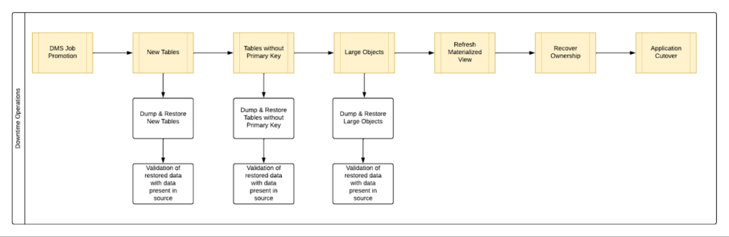
By automating all the downtime operations in this sequential approach, we observed that it took 13 hours for the entire downtime flow to execute for a 1 TB database. This included the migration of 250 MB in new tables, 60 GB in tables without primary keys and 150 GB in large objects.

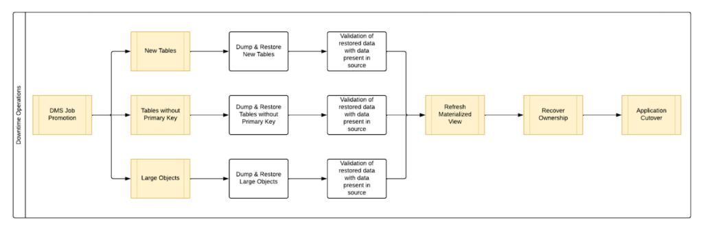
One key observation we made was that, out of all the steps, only three steps took most of the time: migrating new tables, migrating tables without primary keys, and migrating large objects. These took the longest time because they all required dump and restore operations for their respective tables. However, these three steps did not have a hard dependency on each other as they individually targeted different tables. So we tried to run them in parallel as you can see in Fig 2. But the steps following them – ‘Refresh Materialized View’ and ‘Recover Ownership’ – had to be performed sequentially as they targeted the entire database.

However, running these three steps in parallel required upsizing the Cloud SQL instances, as we wanted to have sufficient resources available for each step. This led us to increase the Cloud SQL instances’ vCPU by 50% and memory by 40%, since the export and import operations depended heavily on vCPU consumption as opposed to memory consumption.

Migrating the new tables (created after the DMS job was initiated) and tables without primary keys was straightforward as we were able to leverage the native utilities offered by PostgreSQL – pg_dump and pg_restore. Both utilities process tables in parallel by using multiple threads– the higher the table count, the higher the number of threads that could be executed in parallel, allowing faster migration. With this revised approach, for the same 1 TB database, it still took 12.5 hours for the entire downtime flow to execute.

This improvement reduced the cutover downtime, but we still found that we needed a 12.5 hour window to complete all the steps. We then discovered that 99% of the time of downtime was taken up by just one step: exporting and importing 150 GB of large objects. It turned out that multiple threads could not be used to accelerate the dump and restore large objects in PostgreSQL. Hence, migrating the large objects single handedly extended the downtime for migration by hours. Fortunately, we were able to come up with a workaround for that.

Optimize migration of Large Object from PostgreSQL database

PostgreSQL contains a large objects facility that provides stream-style access to data stored in a special large-object structure. When large objects are stored, they are broken down into multiple chunks and stored in different rows of the database, but are connected under a single Object Identifier (OID). This OID can thus be used to access any stored Large Object. Although users can add large objects to any table in the database, under the hood, PostgreSQL physically stores all large objects within a database in a single table called pg_largeobjects.

While leveraging pg_dump and pg_restore for export and import of large objects, this single table – pg_largeobject, becomes a bottleneck as the PostgreSQL utilities cannot execute multiple threads for parallel processing, since it’s just one table. Typically, the order of operations for these utilities looks something like this:

1. pg_dump reads the data to be exported from the source database
2. pg_dump writes that data into the memory of the client where pg_dump is being executed
3. pg_dump writes from memory to the disk of the the client (a second write operation)
4. pg_restore reads the data from the client’s disk
5. pg_restore writes the data to the destination database

Normally, these utilities would need to be executed sequentially to avoid data loss or data corruption due to conflicting processes. This leads to further increase in migration time for large objects.

Our workaround for this single-threaded process involved two elements. First, with our solution, we eliminated the second write operation – write from memory to disk (point #3). Instead, once the data was read and written into memory, our program would begin the import process and write data to the destination database. Second, since pg_dump and pg_restore could not use multiple threads to process the large objects in just the pg_largeobjects table, we took it upon ourselves to develop a solution that could use multiple threads. The thread count was based on the number of OIDs in the table – pg_largeobjects, and break that single table into smaller chunks for parallel execution.

This approach brought down Large Object migration operation from hours to minutes, therefore bringing down the downtime needed for all operations to be completed that DMS cannot handle, for the same 1 TB database, from 13 hours to just 18 minutes. A reduction of ~98% in the required downtime.

Conclusion

After multiple optimizations and dry runs, we were able to develop a procedure for our client to migrate dozens of terabyte-scale PostgreSQL databases to Google Cloud SQL with a minimal business impact. We developed practices to optimize DMS-based migration by 15% using database flags and reduce downtime by 98% with the help of automation and innovation. These practices can be leveraged for any terabyte-scale migration of PostgreSQL databases to Google Cloud SQL to accelerate migration, minimize downtime and avoid performance impact on mission critical applications.