When you build a data warehouse, the important question is how to ingest data from the source system to the data warehouse. If the table is small you can fully reload a table on a regular basis, however, if the table is large a common technique is to perform incremental table updates. This post demonstrates how you can enhance incremental pipeline performance when you ingest data into BigQuery.

Setting up a standard incremental data ingestion pipeline

We will use the below example to illustrate a common ingestion pipeline that incrementally updates a data warehouse table. Let’s say that you ingest data into BigQuery from a large and frequently updated table in the source system, and you have Staging and Reporting areas (datasets) in BigQuery.

The Reporting area in BigQuery stores the most recent, full data that has been ingested from the source system tables. Usually you create the base table as a full snapshot of the source system table. In our running example, we use BigQuery public data as the source system and create reporting.base_table as shown below. In our example each row is identified by a unique key which consists of two columns: block_hash and log_index.

  CREATE TABLE reporting.base_table  --156 GB processed
PARTITION BY TIMESTAMP_TRUNC(block_timestamp, DAY) AS
SELECT log_index, data, topics, block_timestamp, block_hash
FROM bigquery-public-data.crypto_ethereum.logs
WHERE block_timestamp BETWEEN TIMESTAMP '2020-01-01' AND TIMESTAMP '2020-11-30';

In data warehouses it is common to partition a large base table by a datetime column that has a business meaning. For example, it may be a transaction timestamp, or datetime when some business event happened, etc. The idea is that data analysts who use the data warehouse usually need to analyze only some range of dates and rarely need the full data. In our example, we partition the base table by block_timestamp which comes from the source system.

After ingesting the initial snapshot you need to capture changes that happen in the source system table and update the reporting base table accordingly. This is when the Staging area comes into the picture. The staging table will contain captured data changes that you will merge into the base table. Let’s say that in our source system on a regular basis we have a set of new rows and also some updated records. In our example we mock the staging data as follows: first, we create new data, than we mock the updated records:

  CREATE TABLE staging.load_delta AS --5 GB processed
SELECT log_index, data, topics, block_timestamp, block_hash
FROM bigquery-public-data.crypto_ethereum.logs
WHERE block_timestamp BETWEEN TIMESTAMP '2020-12-01' AND TIMESTAMP '2020-12-07';
 
INSERT INTO staging.load_delta --2 GB processed
SELECT log_index, CONCAT(data, RAND()), topics, block_timestamp, block_hash
FROM bigquery-public-data.crypto_ethereum.logs TABLESAMPLE SYSTEM (5 PERCENT)
WHERE block_timestamp BETWEEN TIMESTAMP '2020-10-01' AND TIMESTAMP '2020-11-30';

Next, the pipeline merges the staging data into the base table. It joins two tables by unique key and than updates the changed value or inserts a new row

  MERGE INTO reporting.base_table T --161 GB processed
USING staging.load_delta S
ON T.block_hash = S.block_hash
 AND T.log_index = S.log_index
WHEN MATCHED THEN UPDATE SET 
  T.data = S.data
WHEN NOT MATCHED THEN INSERT (log_index, data, topics, block_timestamp, block_hash)
VALUES (log_index, data, topics, block_timestamp, block_hash);

It is often the case that the staging table contains keys from various partitions but the number of those partitions are relatively small. It holds, for instance, because in the source system the recently added data may get changed due to some initial errors or ongoing processes but older records are rarely updated. However, when the above MERGE gets executed, BigQuery scans all partitions in the base table and processes 161 GB of data. You might add additional join condition on block_timestamp:

  MERGE INTO reporting.base_table T --161 GB processed
USING staging.load_delta S
ON T.block_hash = S.block_hash
 AND T.log_index = S.log_index
 AND T.block_timestamp = S.block_timestamp
WHEN MATCHED THEN UPDATE SET 
  T.data = S.data
WHEN NOT MATCHED THEN INSERT (log_index, data, topics, block_timestamp, block_hash)
VALUES (log_index, data, topics, block_timestamp, block_hash);

But BigQuery would still scan all partitions in the base table because condition T.block_timestamp = S.block_timestamp is a dynamic predicate and BigQuery doesn’t automatically push such predicates down from one table to another in MERGE.

Can you improve the MERGE efficiency by making it scan less data? The answer is Yes. 

As described in the MERGE documentation, pruning conditions may be located in a subquery filter, a merge_condition filter, or a search_condition filter. In this post we show how you can leverage the first two. The main idea is to turn a dynamic predicate into a static predicate.

Steps to enhance your ingestion pipeline

The initial step is to compute the range of partitions that will be updated during the MERGE and store it in a variable. As was mentioned above, in data ingestion pipelines, staging tables are usually small so the cost of the computation is relatively low.

  DECLARE src_range STRUCT<date_min TIMESTAMP, date_max TIMESTAMP> --115 MB processed
DEFAULT(SELECT STRUCT(
  MIN(block_timestamp) AS date_min,  
  MAX(block_timestamp) AS date_max) FROM staging.load_delta);

Based on your existing ETL/ELT pipeline, you can add the above code as-is to your pipeline or you can compute date_min, data_max as part of some already existing transformation step. Alternatively, date_min, data_max can be computed on the Source System side while capturing the next ingestion data batch.

After computing date_min, date_max you pass those values to the MERGE statement as static predicates. There are several ways to enhance the MERGE and prune partitions in the base table based on precomputed date_min, data_max. 

If your initial MERGE statement uses a subquery, you can incorporate a new filter into it:

  BEGIN 
DECLARE src_range STRUCT<date_min TIMESTAMP, date_max TIMESTAMP> --115 MB processed
DEFAULT(SELECT STRUCT(
  MIN(block_timestamp) AS date_min,  
  MAX(block_timestamp) AS date_max) FROM staging.load_delta);

MERGE INTO reporting.base_table T --41 GB processed
USING (
  SELECT *
  FROM staging.load_delta
  WHERE block_timestamp BETWEEN src_range.date_min AND src_range.date_max) S 
ON T.block_hash = S.block_hash
 AND T.log_index = S.log_index
 AND T.block_timestamp = S.block_timestamp
WHEN MATCHED THEN UPDATE SET 
  T.data = S.data
WHEN NOT MATCHED THEN INSERT (log_index, data, topics, block_timestamp, block_hash)
VALUES (log_index, data, topics, block_timestamp, block_hash);
END;

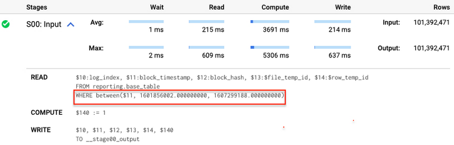
Note that you add the static filter to the staging table and keep T.block_timestamp = S.block_timestamp to convey to BigQuery that it can push that filter to the base table. This MERGE processes 41 GB of data in contrast to the initial 161 GB. You can see in the query plan that BigQuery pushes the partition filter from the staging table to the base table:

This type of optimization, when a pruning condition is pushed from a subquery to a large partitioned or clustered table, is not unique for MERGE. It also works for other types of queries. For instance:

  SELECT * -- 41 GB processed
FROM reporting.base_table T
INNER JOIN staging.load_delta S
ON T.block_hash = S.block_hash
 AND T.log_index = S.log_index
 AND T.block_timestamp = S.block_timestamp
WHERE S.block_timestamp BETWEEN TIMESTAMP '2020-10-05' AND TIMESTAMP '2020-12-07'

And you can check the query plan to verify that BigQuery pushed down the partition filter from one table to another.

Moreover, for SELECT statements, BigQuery can automatically infer a filter predicate on a join column and push it down from one table to another if your query meets the following criteria:

• The target table must be clustered or partitioned. 
• The result size of the other table, i.e. after applying all filters, must qualify for broadcast join. Namly, the result set must be relatively small, less than ~100MB.

In our running example, reporting.base_table is partitioned by block_timestamp. If you define a selective filter on staging.load_delta and join two tables, you can see an inferred filter on the join key pushed to the target table

  SELECT * 
FROM reporting.base_table T
INNER JOIN staging.load_delta S
ON T.block_timestamp = S.block_timestamp
WHERE S.block_hash = '0x0c1caa16b34d94843aabfebc0d5a961db358135988f7498a6fdc450ad55f0870'

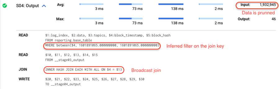
There is no requirement to join tables by partitioning or clustering key to kick off this type of optimization. However, in this case the pruning effect on the target table would be less significant.

But let us get back to the pipeline optimizations. Another way to enhance MERGE is to modify the merge_condition filter by adding static predicate on the base table:

  BEGIN 
DECLARE src_range STRUCT<date_min TIMESTAMP, date_max TIMESTAMP> --115 MB processed
DEFAULT(SELECT STRUCT(
  MIN(block_timestamp) AS date_min,  
  MAX(block_timestamp) AS date_max) FROM staging.load_delta);

MERGE INTO reporting.base_table T --41 GB processed
USING staging.load_delta S
ON T.block_hash = S.block_hash
 AND T.log_index = S.log_index
 AND T.block_timestamp BETWEEN src_range.date_min AND src_range.date_max
WHEN MATCHED THEN UPDATE SET 
  T.data = S.data
WHEN NOT MATCHED THEN INSERT (log_index, data, topics, block_timestamp, block_hash)
VALUES (log_index, data, topics, block_timestamp, block_hash);
END;

To summarize, here are the steps that you can perform to enhance incremental ingestion pipelines in BigQuery. First you compute the range of updated partitions based on the small staging table. Next, you tweak the MERGE statement a bit to let BigQuery know to prune data in the base table.

All the enhanced MERGE statements scanned 41 GB of data, and setting up the src_range variable took 115 MB.  Compare it with the initial 161 GB scan. Moreover, given that computing src_range may be incorporated into some existing transformation in your ETL/ELT, it results in a good performance improvement which you can leverage in your pipelines. 

In this post we described how to enhance data ingestion pipelines by turning dynamic filter predicates into static predicates and letting BiQuery prune data for us. You can find more tips on BigQuery DML tuning here.

Special thanks to Daniel De Leo, who helped with examples and provided valuable feedback on this content.

Organizations today build data lakes to process, manage and store large amounts of data that  originate from different sources both on-premise and on cloud. As part of their data lake strategy, organizations want to leverage some of the leading OSS frameworks such as Apache Spark for data processing, Presto as a query engine and Open Formats for storing data such as Delta Lake for the flexibility to run anywhere and avoiding lock-ins.

Traditionally, some of the major challenges with building and deploying such an architecture were:

• Object Storage was not well suited for handling mutating data and engineering teams spent a lot of time in building workarounds for this
• Google Cloud provided the benefit of running Spark, Presto and other varieties of clusters with the Dataproc service, but one of the challenges with such deployments was the lack of a central Hive Metastore service which allowed for sharing of metadata across multiple clusters.
• Lack of integration and interoperability across different Open Source projects

To solve for these problems, Google Cloud and the Open Source community now offers:

• Native Delta Lake support in Dataproc, a managed OSS Big Data stack for building a data lake with Google Cloud Storage, an object storage that can handle mutations
• A managed Hive Metastore service called Dataproc Metastore which is natively integrated with Dataproc for common metadata management and discovery across different types of Dataproc clusters
• Spark 3.0 and Delta 0.7.0 now allows for registering Delta tables with the Hive Metastore which allows for a common metastore repository that can be accessed by different clusters.

Architecture

Here’s what a standard Open Cloud Datalake deployment on GCP might consist of:

1. Apache Spark running on Dataproc with native Delta Lake Support
2. Google Cloud Storage as the central data lake repository which stores data in Delta format
3. Dataproc Metastore service acting as the central catalog that can be integrated with different Dataproc clusters
4. Presto running on Dataproc for interactive queries

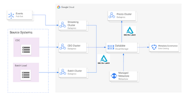
Such an integration provides several benefits:

1. Managed Hive Metastore service
2. Integration with Data Catalog for data governance
3. Multiple ephemeral clusters with shared metadata
4. Out of the box integration with open file formats and standards

Reference implementation

Below is a step by step guide for a reference implementation of setting up the infrastructure and running a sample application

Setup

The first thing we would need to do is set up 4 things:

1. Google Cloud Storage bucket for storing our data
2. Dataproc Metastore Service
3. Delta Cluster to run a Spark Application that stores data in Delta format
4. Presto Cluster which will be leveraged for interactive queries

Create a Google Cloud Storage bucket

Create a Google Cloud Storage bucket with the following command using a unique name.

  gsutil mb gs://<your-bucket-name>

Create a Dataproc Metastore service

Create a Dataproc Metastore service with the name “demo-service” and with version 3.1.2. Choose a region such as us-central1. Set this and your project id as environment variables.

  REGION=<your-region>
PROJECT_ID=<your-project-id>
gcloud metastore services create demo-service \
    --hive-metastore-version=3.1.2 \
    --location=${REGION}

Create a Dataproc cluster with Delta Lake

Create a Dataproc cluster which is connected to the Dataproc Metastore service created in the previous step and is in the same region. This cluster will be used to populate the data lake. The jars needed to use Delta Lake are available by default on Dataproc image version 1.5+

  gcloud dataproc clusters create delta-cluster \
    --dataproc-metastore=projects/${PROJECT_ID}/locations/us-central1/services/demo-service \
    --region=${REGION} \
    --image-version=2.0.0-RC22-debian10

Create a  Dataproc cluster with Presto 

Create a Dataproc cluster in us-central1 region with the Presto Optional Component and connected to the Dataproc Metastore service.

  gcloud dataproc clusters create presto-cluster \
    --dataproc-metastore=projects/${PROJECT_ID}/locations/us-central1/services/demo-service \
    --region=${REGION} \
    --image-version=2.0-debian10 \
    --optional-components=PRESTO \
    --enable-component-gateway

Spark Application

Once the clusters are created we can log into the Spark Shell by SSHing into the master node of our Dataproc cluster “delta-cluster”.. Once logged into the master node the next step is to start the Spark Shell with the delta jar files which are already available in the Dataproc cluster. The below command needs to be executed to start the Spark Shell. Then, generate some data.

  spark-shell --jars /usr/lib/delta/jars/delta-core.jar
import io.delta.tables._
import org.apache.spark.sql.functions._
// Simulate application data
val orig_df = Seq(
  (1L, 3.0), (2L, -1.0), (3L, 0.0)
).toDF("x", "y")

# Write Initial Delta format to GCS

Write the data to GCS with the following command, replacing the project ID.

  orig_df.write.mode("append").format("delta").save("gs://<your-bucket-name>/first-delta-table")

# Ensure that data is read properly from Spark

Confirm the data is written to GCS with the following command, replacing the project ID.

  spark.read.format("delta").load("gs://<your-bucket-name>/first-delta-table").show()

Once the data has been written we need to generate the manifest files so that Presto can read the data once the table is created via the metastore service.

# Generate manifest files

  val deltaTable = DeltaTable.forPath("gs://<your-bucket-name>/first-delta-table")
deltaTable.generate("symlink_format_manifest")

With Spark 3.0 and Delta 0.7.0 we now have the ability to create a Delta table in Hive metastore. To create the table below command can be used. More details can be found here 

# Create Table in Hive metastore

  spark.sql("CREATE TABLE my_first_table (x bigint,y double) ROW FORMAT SERDE 'org.apache.hadoop.hive.ql.io.parquet.serde.ParquetHiveSerDe' STORED AS INPUTFORMAT 'org.apache.hadoop.hive.ql.io.SymlinkTextInputFormat' OUTPUTFORMAT 'org.apache.hadoop.hive.ql.io.HiveIgnoreKeyTextOutputFormat' LOCATION 'gs://<your-bucket-name>/first-delta-table/_symlink_format_manifest'")

Once the table is created in Spark, log into the Presto cluster in a new window and verify the data. The steps to log into the Presto cluster and start the Presto shell can be found here.

#Verify Data in Presto

  presto:default> select * from hive.default.my_first_table;
 x  |  y  
----+------
  2 | -1.0
  3 |  0.0
  1 |  3.0

Once we verify that the data can be read via Presto the next step is to look at schema evolution. To test this feature out we create a new dataframe with an extra column called “z” as shown below:

# Schema Evolution in Spark

Switch back to your Delta cluster’s Spark shell and enable the automatic schema evolution flag

  spark.sql("SET spark.databricks.delta.schema.autoMerge.enabled = true")

Once this flag has been enabled  create a new dataframe that has a new set of rows to be inserted along with a new column 

  val merge_df = Seq(
  (10L, 30.0, "a"), (20L, -10.0, "b"), (30L, 100.0, "c")
).toDF("x", "y", "z")

Once the dataframe has been created we leverage the Delta Merge function to UPDATE existing data and INSERT new data 

# Use Delta Merge Statement to handle automatic schema evolution and add new rows

  deltaTable.alias("o").merge(merge_df.as("n"),"o.x = n.x").whenMatched.updateAll().whenNotMatched.insertAll().execute()

As a next step we would need to do two things for the data to reflect in Presto:

1. Generate updated schema manifest files so that Presto is aware of the updated data
2. Modify the table schema so that Presto is aware of the new column.

When the data in a Delta table is updated you must regenerate the manifests using either of the following approaches:

• Update explicitly: After all the data updates, you can run the generate operation to update the manifests.
• Update automatically: You can configure a Delta table so that all write operations on the table automatically update the manifests. To enable this automatic mode, you can set the corresponding table property using the following SQL command.

  ALTER TABLE delta.<path-to-delta-table> SET TBLPROPERTIES(delta.compatibility.symlinkFormatManifest.enabled=true)

However, in this particular case we will use the explicit method to generate the manifest files again

  deltaTable.generate("symlink_format_manifest")

Once the manifest file has been re-created the next step is to update the schema in Hive metastore for Presto to be aware of the new column. This can be done in multiple ways, one of the ways to do this is shown below:

# Promote Schema Changes via Delta to Presto

  val schema_evolution = "ALTER TABLE my_first_table ADD COLUMN ( " + merge_df.schema.toDDL.replace(orig_df.schema.toDDL,"").substring(1) + ")"
spark.sql(s"$schema_evolution")

Once these changes are done we can now verify the new data and new column in Presto as shown below:

# Verify changes in Presto

  presto:default> select * hive.default.from my_first_table;
 x  |   y   |  z  
----+-------+------
 20 | -10.0 | b    
  2 |  -1.0 | NULL
  3 |   0.0 | NULL
 30 | 100.0 | c    
 10 |  30.0 | a    
  1 |   3.0 | NULL

In summary, this article demonstrated:

1. Set up the Hive metastore service using Dataproc Metastore, spin up Spark with Delta lake and Presto clusters using Dataproc
2. Integrate the Hive metastore service with the different Dataproc clusters
3. Build an end to end application that can run on an OSS Datalake platform powered by different GCP services

Next steps

If you are interested in building an Open Data Platform on GCP please look at the Dataproc Metastore service for which the details are available here and for details around the Dataproc service please refer to the documentation available here. In addition, refer to this blog which explains in detail the different open storage formats such as Delta & Iceberg that are natively supported within the Dataproc service.