So far on the BigQuery Admin Reference Guide series, we’ve talked about the different logical resources available inside of BigQuery. Now, we’re going to begin talking about BigQuery’s architecture. In this post we’re diving into how BigQuery stores your data in native storage, and what levers you can pull to optimize how your data is stored. 

Columnar storage format

BigQuery offers fully managed storage, meaning you don’t have to provision servers. Sizing is done automatically and you only pay for what you use. Because BigQuery was designed for large scale data analytics data is stored in columnar format.

Traditional relational databases, like Postgres and MySQL, store data row-by-row in record-oriented storage. This makes them great for transactional updates and OLTP (Online Transaction Processing) use cases because they only need to open up a single row to read or write data. However, if you want to perform an aggregation like a sum of an entire column, you would need to read the entire table into memory.

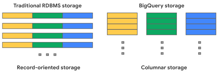
BigQuery uses columnar storage where each column is stored in a separate file block. This makes BigQuery an ideal solution for OLAP (Online Analytical Processing) use cases. When you want to perform aggregations you only need to read the column that you are aggregating over.

Optimized storage format

Internally, BigQuery stores data in a proprietary columnar format called Capacitor. We know Capacitor is a column-oriented format as discussed above. This means that the values of each field, or column,  are stored separately so the  overhead of reading the file is proportional to the number of fields you actually read. This doesn’t necessarily mean that each column is in its own file, it just means that each column is stored in a file block, which is actually compressed independently for increased optimization.

What’s really cool is that Capacitor builds an approximation model that takes in relevant factors like the type of data (e.g. a really long string vs. an integer) and usage of the data (e.g. some columns are more likely to be used as filters in WHERE clauses) in order to reshuffle rows and encode columns. While every column is being encoded, BigQuery also collects various statistics about the data — which are persisted and used later during query execution.

If you want to learn more about Capacitor, check out this blog post from Google’s own Chief BigQuery Officer. 

Encryption and managed durability

Now that we understand how the data is saved in specific files, we can talk about where these files actually live. BigQuery’s persistence layer is provided by Google’s distributed file system, Colossus, where data is automatically compressed, encrypted, replicated, and distributed.

There are many levels of defense against unauthorized access in Google Cloud Platform, one of them being that 100% of data is encrypted at rest. Plus, if you want to control encryption yourself, you can use customer-managed encryption keys.

Colossus also ensures durability by using something called erasure encoding – which breaks data into fragments and saves redundant pieces across a set of different disks.  However, to ensure the data is both durable and available, the data is also replicated to another availability zone within the same region that was designated when you created your dataset.

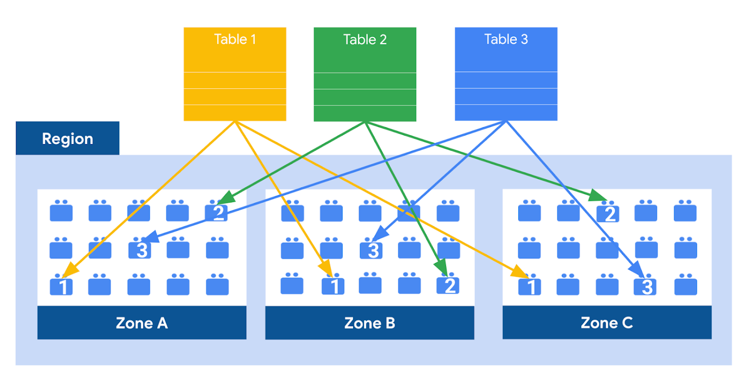
This means data is saved in a different building that has a different power system and network. The chances of multiple availability zones going offline at once is very small. But if you use “Multi-Region” locations – like the US or EU – BigQuery stores another copy of the data in an off-region replica. That way, the data is recoverable in the event of a major disaster.

This is all accomplished without impacting the compute resources available for your queries. Plus encoding, encryption and replication are included in the price of BigQuery storage – no hidden costs!

Optimizing storage for query performance

BigQuery has a built-in storage optimizer that helps arrange data into the optimal shape for querying, by periodically rewriting files. Files may be written first in a format that is fast to write but later BigQuery will format them in a way that is fast to query. Aside from the optimization happening behind the scenes, there are also a few things you can do to further enhance storage.

Partitioning

A partitioned table is a special table that is divided into segments, called partitions. BigQuery leverages partitioning to minimize the amount of data that workers read from disk. Queries that contain filters on the partitioning column can dramatically reduce the overall data scanned, which can yield improved performance and reduced query cost for on-demand queries. New data written to a partitioned table is automatically delivered to the appropriate partition.

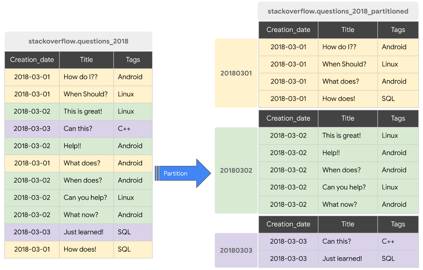
BigQuery supports the following ways to create partitioned tables:

• Ingestion time partitioned tables: daily partitions reflecting the time the data was ingested into BigQuery. This option is useful if you’ll be filtering data based on when new data was added. For example, the new Google Trends Dataset is refreshed each day, you might only be interested in the latest trends. 
• Time-unit column partitioned tables: BigQuery routes data to the appropriate partition based on date value in the partitioning column. You can create partitions with granularity starting from hourly partitioning. This option is useful if you’ll be filtering data based on the date value in the table, for example looking at the most recent transactions by including a WHERE clause for transaction_created_date
• INTEGER range partitioned tables: Partitioned based on an integer column  that can be bucketed. This option is useful if you’ll be filtering data based on an integer column in the table, for example focusing on specific customers using customer_id. You can bucket the integer values to create appropriately sized partitions, like having all customers with IDs from 0-100 in the same partition. 

Partitioning is a great way to optimize query performance, especially for large tables that are often filtered down during analytics. When deciding on the appropriate partition key, make sure to consider how everyone in your organization is leveraging the table. For large tables that could cause some expensive queries, you might want to require partitions to be used.

Partitions are designed for places where there is a large amount of data and a low number of distinct values. A good rule of thumb is making sure partitions are greater than 1 GB. If you over partition your tables, you’ll create a lot of metadata – which means that reading in lots of partitions may actually slow down your query. 

Clustering

When a table is clustered in BigQuery, the data is automatically sorted based on the contents of one or more columns (up to 4, that you specify). Usually high cardinality and non-temporal columns are preferred for clustering, as opposed to partitioning which is better for fields with lower cardinality. You’re not limited to choosing just one, you can have a single table that is both partitioned and clustered!

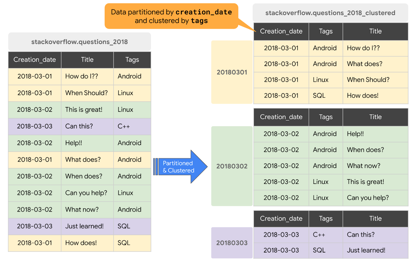
The order of clustered columns determines the sort order of the data. When new data is added to a table or a specific partition, BigQuery performs free, automatic re-clustering in the background. Specifically, clustering can improve the performance for queries:

• Containing where clauses with a clustered column: BigQuery uses the sorted blocks to eliminate scans of unnecessary data. The order of the filters in the where clause matters, so use filters that leverage clustering first
• That aggregate data based on values in a clustered column: performance is improved because the sorted blocks collocate rows with similar values
• With joins where the join key is used to cluster the table: less data is scanned, for some queries this offers a performance boost over partitioning!

Looking for some more information and example queries? Check out this blog post! 

Denormalizing

If you come from a traditional database background, you’re probably used to creating normalized schemas – where you optimize your structure so that data is not repeated. This is important for OLTP workloads (as we discussed earlier) because you’re often making updates to the data. If your customer’s address is stored every place they have made a purchase, then it might be cumbersome to update their address if it changes. 

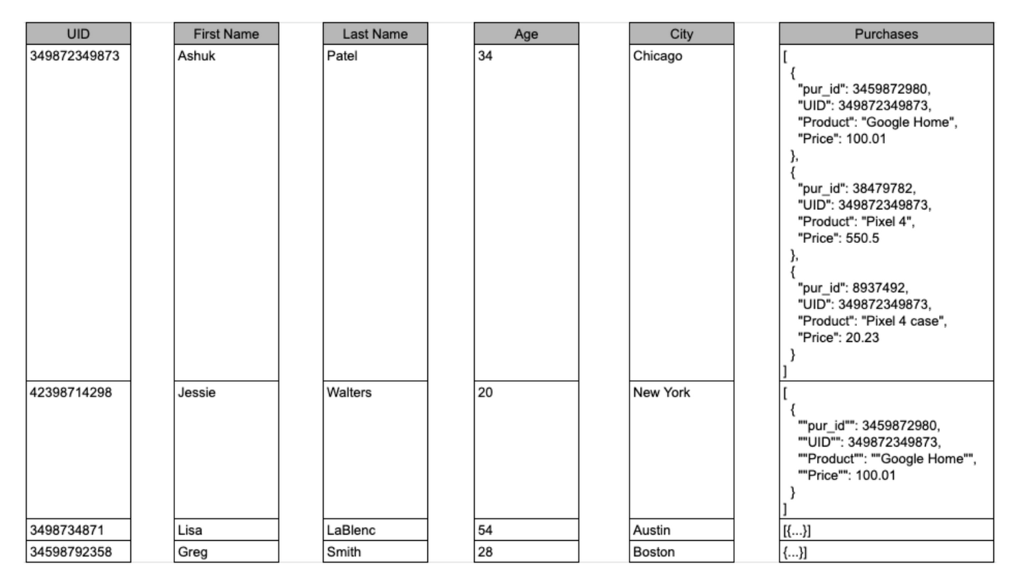
However, when performing analytical operations on normalized schemas, usually multiple tables need to be joined together. If we instead denormalize our data, so that information (like the customer address) is repeated and stored in the same table, then we can eliminate the need to have a JOIN in our query. For BigQuery specifically, we can also take advantage of support for nested and repeated structures. Expressing records using STRUCTs and ARRAYs can not only provide a more natural representation of the underlying data, but in some cases it can also eliminate the need to use a GROUP BY statement. For example, using ARRAY_LENGTH instead of COUNT.

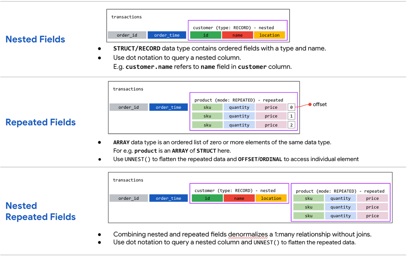
Keep in mind that denormalization has some disadvantages. First off, they aren’t storage-optimal. Although, many times the low cost of BigQuery storage addresses this concern. Second, maintaining data integrity can require increased machine time and sometimes human time for testing and verification. We recommend that you prioritize partitioning and clustering before denormalization, and then focus on data that rarely requires updates. 

Optimizing for storage costs

When it comes to optimizing storage costs in BigQuery, you may want to focus on removing unneeded tables and partitions. You can configure the default table expiration for your datasets, configure the expiration time for your tables, and configure the partition expiration for partitioned tables. This can be especially useful if you’re creating materialized views or tables for ad-hoc workflows, or if you only need access to the most recent data.

Additionally, you can take advantage of BigQuery’s long term storage. If you have a table that is not used for 90 consecutive days, the price of storage for that table automatically drops by 50 percent to $0.01 per GB, per month. This is the same cost as Cloud Storage Nearline, so it might make sense to keep older, unused data in BigQuery as opposed to exporting it to Cloud Storage.Thanks for tuning in this week! Next week, we’re talking about query processing – a precursor to some query optimization techniques that will help you troubleshoot and cut costs.  Be sure to stay up-to-date on this series by following me on LinkedIn and Twitter!

As software-defined vehicles continue to advance and the quantity of digital services grows to meet consumer demand, the data required to provide these services continue to grow as well. This makes automotive manufacturers and suppliers look for capabilities to log and analyze data, update applications, and extend commands to in-vehicle software.

The challenges the automotive sector faces can be quantified. A modern vehicle contains upwards of 70 electronic control units (ECUs), most of which are connected to one or more sensors. Not only is it now possible to exactly measure many aspects of vehicle performance, but new options become available. Using LIDAR (light detection and ranging), for example, vehicles are achieving higher levels of autonomy; this leads to a data stream from such demanding applications that may reach 25 GB per hour. For the in-vehicle processing of data, 100 million lines of software code may be present — more than a fighter jet. This in-vehicle code will have to be maintained with updates and new functionalities.

Access to the data will allow manufacturers to gain valuable insights into operational details of their vehicles. The use of this data can help to reduce costs and risks, increase ROI, support ESG initiatives, and provide valuable insights to develop innovative solutions and shorten the time to value for Electric Vehicle innovations.

Sibros’ Deep Connected Platform (DCP) makes it possible for these manufacturers to build and launch new connected vehicle use cases from production to post-sale at scale by connecting and managing all software and data throughout every life cycle stage. A key component of this platform is the Sibros Deep Logger that provides capabilities like the following:

• Full configurability of what to record, when to record it, and how fast to record it.
• High resolution timestamps of all Controller Area Network (CAN) messages.
• Dynamic application of live log configurations to receive new data points without deploying new software.

For example, properly analyzed engine data enables true predictive maintenance for the first time, which creates the option to repair or replace components before failure happens. Another example would be the evaluation of data regarding the use of certain in-car features with the goal to redesign its interior.

Two other components of the DCP are software updates and remote commands to ECUs. The DCP on Google Cloud enables seamless integration with any vehicle architecture and provides OEMs and suppliers with the platform to manage connected vehicle data at rest and in transit using a proven and secure way on a global scale.

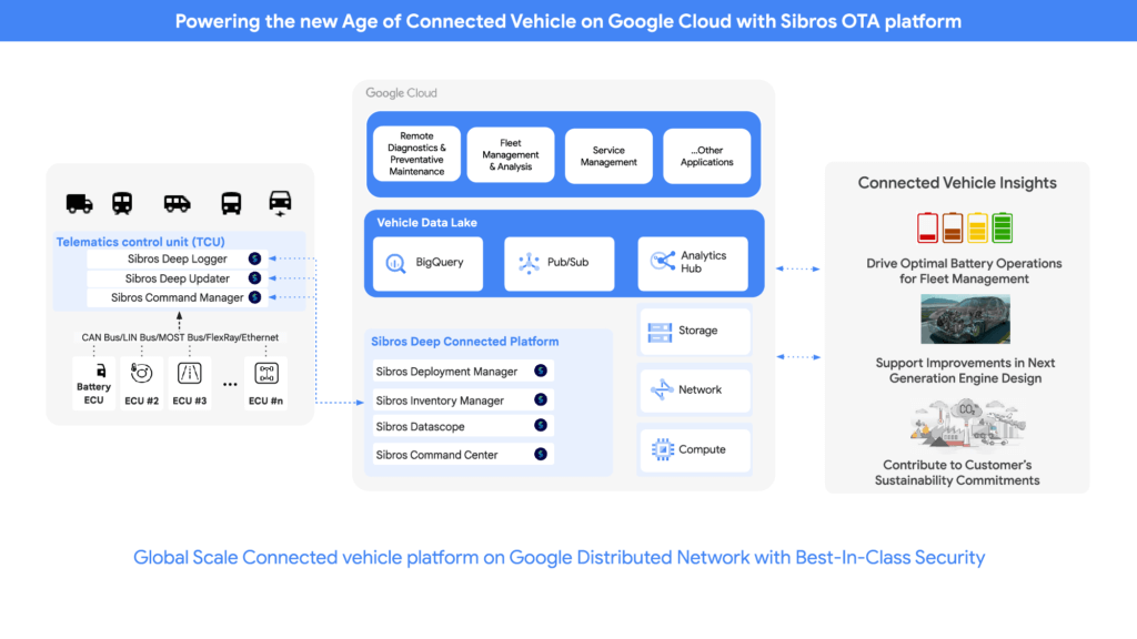
OEMs can pull data through APIs provided by Sibros into Google Data Cloud (including BigQuery) to gain access to the rich information data sets provided by the DCP within their environment and blend this data with their first party data sets to provide value insights for their business. Some of the Connected Vehicle insights that DCP information enables are:

• Damage prevention, improved operation, or development of the next generation of engines with insights from complex analyses that could consider parameters like model, engine type, mileage, overall speed, temperature, air pressure, load, services, and more.
• The combination of electric vehicle battery usage data like charging cycles, engine performance, and battery age with contributing factors as the use of the air conditioning to determine if such factors contribute to hazardous battery conditions and for improved battery development.
• Cross-organization collaboration in R&D by the provision of information on all these metrics and more from real-world driving, like engine knock data and even tire pressure.
• Google Cloud’s unified data cloud offering provides a complete platform for building data-driven applications like those from Sibros — from simplified data ingestion, processing, and storage to powerful analytics, AI, ML, and data sharing capabilities — integrated with Google Cloud. With a diverse partner ecosystem and support for multi-cloud, open-source tools and APIs, Google Cloud provides Sibros the portability and the extensibility they need to avoid data lock-in.

“Software has an ever increasing importance in the automotive world, even more so with electric vehicles and new mobility services. Google Cloud is partnering with Sibros to bring their award winning Deep Connected Platform to deliver high frequency, low latency over-the-air software updates, data logging & diagnostics capabilities to our automotive customers, leveraging the security and scale of Google Cloud. This is revolutionizing everything from development cycles to business models and customer relationships.” — Matthias Breunig, Director, Global Automotive Solutions, Google Cloud

Through Built with BigQuery, Google Cloud is helping tech companies like Sibros build innovative applications on Google’s Data Cloud with simplified access to technology, helpful and dedicated engineering support, and joint go-to-market programs.

“Sibros is looking forward to partnering with Google Cloud, which will enable vehicle manufacturers and suppliers to reach the next level in their use of data. Sibros solutions for Deep Data Logging and Updating on the Google Data Cloud, combined with Google BigQuery, will help them to mitigate risks, reduce costs, add innovative products, and introduce value-added use cases.” — Xiaojian Huang, Chief Digital Officer, Software, Sibros

Sibros and Google Cloud are driving Connected Mobility transformation to help our customers accelerate R&D innovation, power efficient operations, and unlock software-defined vehicle use cases with a full stack connected vehicle platform. Click here to learn more about Sibros on Google Cloud.

Mercury, the Roman god of commerce, is often depicted carrying a purse, symbolic of business transactions, wearing winged sandals, illustrating his abilities to move at great speeds. Transactions power the world’s business systems today, ranging from millions of packages moving worldwide tracked in real time by logistics companies to global payments from personal loans to securities trading to intergovernmental transactions, keeping goods and services flowing worldwide. Today, we are very pleased to announce the public preview of multi-statement transactions in BigQuery.

BigQuery has long supported single-statement transactions through DML statements such as INSERT, UPDATE, DELETE, MERGE and TRUNCATE, applied to one table per transaction. Multi-statement transactions expand on this scope by supporting multiple SQL statements, including DML, spanning multiple tables in a single transaction. This means that the changes to data across multiple tables associated with all statements in a given transaction are committed atomically (all at once) if successful or all rolled back atomically in the event of a failure. These new multi-statement transaction capabilities now bridge the gap between online transaction processing (OLTP) systems and BigQuery through tighter and faster integration, just as Mercury’s speed enabled him to travel rapidly between the mortal and divine worlds.

Overview

A transaction is a set of tasks carried out against a database or a data warehouse representing a business unit of work. For example, an order expedite action may result in a series of changes to multiple tables, e.g., updating delivery dates on the order, adding new shipment lines on a shipment to create expedited delivery shipments and canceling (updating) prior normal delivery shipment lines. Correspondingly, when a batch job execute an ETL process in a data warehouse, it may perform data wrangling and data cleansing operations by transforming and saving the data in multiple tables. In both of these cases, if a failure occurs, then the entire transaction must be rolled back so that the system of record does not have partial data saved putting the dataset in an inconsistent state.

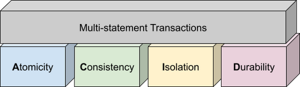
Transactions are known for their atomicity, consistency, isolation, and durability (ACID) properties. Atomicity indicates that all data changes (including metadata changes) are applied or reverted in a single operation, e.g. when a set of rows are added to a table with enrichment and the corresponding set of rows deleted, both operations happen together. Consistency refers to the consistency of data before and after the transaction has completed. When data is added to or updated in a table, the changes to data in tables are consistent with the constraints specified on the table or its columns, e.g. ensuring that the NOT NULL constraint is complied with when data gets added or modified in a table. Isolation indicates that multiple transactions can make changes to the table concurrently as long as the changes don’t conflict with each other, e.g. two transactions loading data into tables from different business units can proceed concurrently. Durability is the last and possibly the most important property of transactions which guarantees that in the event of a failure (after completing the transaction), all the changes committed by the transaction are saved for future transactions or queries.

Isolation level

All transactions in BigQuery including multi-statement transactions support snapshot isolation. At this isolation level, all statements in a transaction see a consistent snapshot of the database, as of the start of the transaction. BigQuery achieves this due to its multi-version property where it maintains the history of mutations to the database for a certain period. Transactions do not see any changes, committed or uncommitted, from other concurrent transactions while the transaction is in progress. BigQuery supports read-your-own-writes, where statements in a transaction can see all the changes applied by prior statements in the same transaction.

Example

Let’s run through an example to demonstrate how BigQuery supports the concept of multi-statement transactions with multiple sets of changes across multiple tables in one operation. In this example, we will set up this demo by creating 10 tables each with 100 partitions 

Language: SQL

  DECLARE num_tables DEFAULT 10;
DECLARE x INT64 DEFAULT 0;
# replace "demo" with your preferred dataset name
DECLARE ds STRING default "`00jathreya`";
DECLARE prefix STRING DEFAULT "mst_demo";
DECLARE table_name STRING;
DECLARE pre_table_name STRING;
/*
Sets up 10 tables, with schema (partition_id:integer,value:timestamp).
Each table has 100 partitions, with partition key 0, 10, 20, ..., 990.
*/
SET x = 0;
WHILE x < num_tables DO
 SET table_name = format("%s.%s_%d", ds, prefix, x); 
 EXECUTE IMMEDIATE format("""DROP TABLE IF EXISTS %s""", table_name); 
 EXECUTE IMMEDIATE format("""
 CREATE OR REPLACE TABLE %s (partition_id INT64, value TIMESTAMP)
 PARTITION BY RANGE_BUCKET(partition_id, GENERATE_ARRAY(0, 1000, 10))
 AS SELECT partition_id, CURRENT_TIMESTAMP() AS value FROM UNNEST(GENERATE_ARRAY(0, 990, 10)) AS partition_id
 """, table_name);
 SET x = x + 1;
END WHILE;
# Verify the partitioned tables created and the timestamp
execute immediate format("""select table_schema, table_name, count(partition_id), sum(total_rows), max(last_modified_time) from %s.INFORMATION_SCHEMA.PARTITIONS
where starts_with(table_name,'%s')
group by table_schema, table_name""", ds, prefix);
# Verify data in table 9 based on the timestamp
EXECUTE IMMEDIATE format("""
SELECT * FROM %s ORDER BY partition_id
""", table_name);

Next, we will show how the new COMMIT and ROLLBACK commands in BigQuery allow you to save or reverse the changes in a transaction spanning multiple tables.

Language: SQL

  DECLARE num_tables DEFAULT 10;
DECLARE x INT64 DEFAULT 0;
# Replace `mydataset` with your preferred dataset name
DECLARE ds STRING DEFAULT "`mydataset`";
DECLARE prefix STRING DEFAULT "mst_demo";
DECLARE table_name STRING;
DECLARE pre_table_name STRING;
/*
Steps of the transaction:
1. For table 0, updates the timestamp to CURRENT_TIMESTAMP.
2. FOR table 1 to 9, merge table x using data from table x-1. All MERGE should
see the updated data in table x-1, so as a result the change in table 0 should be
propagated all the way to table 9.
3. A total of 1000 partition changes on 10 tables.
*/
BEGIN TRANSACTION;
SET x = 0;
WHILE x < num_tables DO
 SET table_name = format("%s.%s_%d", ds, prefix, x);
 IF x = 0 THEN
   EXECUTE IMMEDIATE format("""
   UPDATE %s SET value = CURRENT_TIMESTAMP WHERE true
   """, table_name);
 ELSE
   SET pre_table_name = format("%s.%s_%d", ds, prefix, x-1);
   EXECUTE IMMEDIATE format("""
   MERGE %s t2 USING %s t1 ON t2.partition_id = t1.partition_id
   WHEN MATCHED THEN UPDATE SET value = t1.value
   """, table_name, pre_table_name);
 END IF;
 SET x = x + 1;
END WHILE;
# Verify data in table 9 inside transaction shows recently updated data
SET table_name = format("%s.%s_%d", ds, prefix, num_tables-1);
EXECUTE IMMEDIATE format("""
SELECT * FROM %s ORDER BY partition_id
""", table_name);
IF x = 9 THEN
 COMMIT TRANSACTION;
ELSE
 ROLLBACK TRANSACTION;
END IF;
# Verify data in table 9 outside transaction shows timestamp of original data
EXECUTE IMMEDIATE format("""
SELECT * FROM %s ORDER BY partition_id
""", table_name);

Monitoring and Management

Unlike single-statement transactions which map to a single DML command, multi-statement transactions are complex spanning multiple DML operations across multiple tables. To monitor these complex jobs, the BigQuery JOBS INFORMATION_SCHEMA views have been expanded to add a new column, TRANSACTION_ID, which contains a unique identifier for each transaction in BigQuery. You can query transactions that are in progress or the ones that have completed by querying these views.

Language: SQL

  #Returns the list of transactions running under a parent job ID .;
SELECT
DISTINCT transaction_id
FROM `region-us`.INFORMATION_SCHEMA.JOBS_BY_PROJECT
WHERE parent_job_id = "job_id" AND state = "RUNNING";
# Returns the active transactions and parent job id that are running and affect a named table.;
WITH 
  running_transactions AS (
  SELECT DISTINCT transaction_id 
  FROM `region-us`.INFORMATION_SCHEMA.JOBS_BY_PROJECT 
  WHERE state = "RUNNING")
SELECT 
  transaction_id, parent_job_id, query 
FROM `region-us`.INFORMATION_SCHEMA.JOBS_BY_PROJECT, running_transactions
WHERE destination_table = "mytable" 
  AND transaction_id = running_transactions.transaction_id;
# Returns all successfully committed transactions
SELECT 
  transaction_id, parent_job_id, query 
FROM `region-us`.INFORMATION_SCHEMA.JOBS_BY_PROJECT 
WHERE statement_type = "COMMIT_TRANSACTION" AND error_result IS NULL;
# Returns all rolled back transactions
SELECT 
  transaction_id, parent_job_id, query 
FROM `region-us`.INFORMATION_SCHEMA.JOBS_BY_PROJECT
WHERE statement_type = "ROLLBACK_TRANSACTION" AND error_result IS NULL;

To terminate a transaction, you will need to terminate the parent job under which the transaction is running by passing the parent job ID of the script containing the transaction to the BQ.JOBS.CANCEL system procedure.

Conclusion

As enterprises accelerate towards more real time insight-driven decisions, multi-statement transactions are a key enabler towards bringing transaction data into analytical data warehouses, such as BigQuery. With strong ACID properties, full transaction support for commit and rollback, and rich monitoring and management APIs built on proven transaction processing backbone, we are very pleased to help our BigQuery customers unlock the value of transactions through these new capabilities.

Database disaster recovery (DR) planning is an important component of a bigger DR plan, and for enterprises using Microsoft SQL Server on Compute Engine, it often involves critical data.

When you’re architecting a disaster recovery solution with Microsoft SQL Server running on Google Cloud Platform (GCP), you have some decisions to make to build an effective, comprehensive plan. 

Microsoft SQL Server includes a variety of disaster recovery strategies and features, such as Always On availability groups or Failover Cluster Instances.

And Google Cloud is designed from the start for resilience and availability. There are several types of data centers available within GCP where you can map SQL Server’s availability features based on your specific requirements: zones and regions. Zones are autonomous data centers co-located within a GCP region. These regions are available in different geographies such as North America or APAC. 

However, there is no single disaster recovery strategy to map Microsoft SQL Server DR features to Google Cloud’s data center topology that satisfies every possible combination of disaster recovery requirements.

As a database architect, you have to design a custom disaster recovery strategy based on your specific use cases and requirements.

Our new Disaster Recovery for Microsoft SQL Server solution provides information on Microsoft’s SQL Server disaster recovery strategies, and shows how you can map them to zones and regions in GCP based on your business’s particular criteria and requirements. One example is deploying an availability group within a region across three zones (shown in the diagram below). 

For successful DR planning, you should have a clear conceptual model and established terminology in place. In this solution, you’ll find a base set of concepts and terms in context of Google Cloud DR. This includes defining terms like primary database, secondary database, failover, switchover, and fallback.

You’ll also find details on recovery point objective, recovery time objective and single point of failure domain, since those are key drivers for developing a specific disaster recovery solution.

Building a DR solution with Microsoft SQL Server in GCP regions
To get started with implementing the availability features of Microsoft SQL Server in the context of Google Cloud, take a look at this diagram, which shows the implementation of an Always On availability group in a GCP region, using several zones:

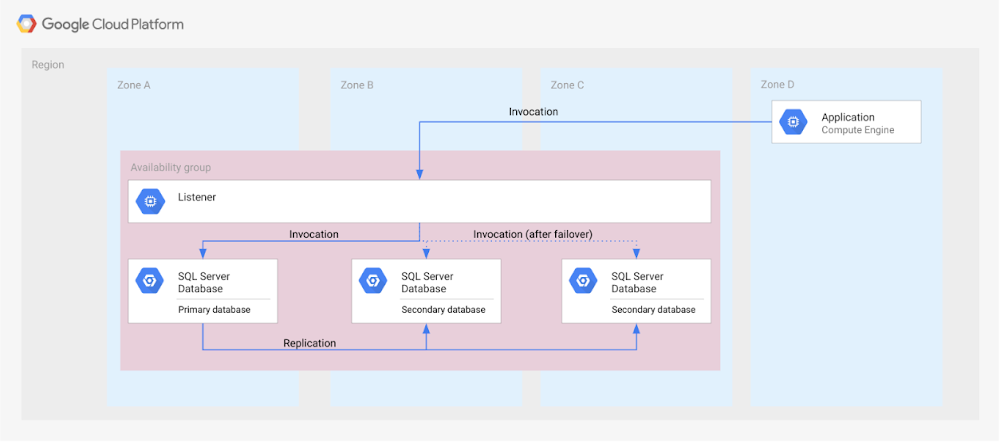
In the new solution, you’ll see other availability features, like log shipping, along with how they map to GCP. In addition, features in Microsoft SQL Server that are not deemed availability features—like server replication and backup file shipping—can actually be used for disaster recovery, so those are included as well. 

Disaster recovery features of Microsoft SQL Server do not have to be used in isolation and can be combined for more complex and demanding use cases. For example, you can set up availability groups in two regions with log shipping as the transfer mechanism between the regions.

Disaster Recovery for Microsoft SQL Server also describes the disaster recovery process itself, how to test and verify a defined disaster recovery solution, and outlines a basic approach, step-by-step.