






Accelerate Innovation with Google Cloud’s Managed Database Services
READ FULL INTRODOWNLOAD AGAIN1277
Of your peers have already downloaded this article
4:30 Minutes
The most insightful time you'll spend today!
Cart.com to Transform e-Commerce for Brands Globally

8748
Of your peers have already read this article.
1:30 Minutes
The most insightful time you'll spend today!
The ecommerce playing field has been hard to navigate for most retailers, and Cart.com is on a mission to change that. Traditionally, retailers needing to run their online store, order fulfillment, customer service, marketing, and other essential activities have had to cobble together systems to get the capabilities they need – much less having access to analytics across these functions. The result is costly, siloed ecommerce operations that are difficult to manage and scale.
It’s clearly not a formula for success, yet that’s the reality facing most retailers. Cart.com, in contrast, has set out to democratize ecommerce by giving brands of all sizes the full capabilities they need to take on the world’s largest online retailers. Our end-to-end environment empowers retailers to keep more of their revenue, set up proven strategies for managing all aspects of their business, and act on valuable insights from customer data every step of the way.
Together with our talented team, we’re building a unified ecommerce platform that already provides value to many leading or up and coming brands including Whataburger, GUESS, Dr. Scholl’s, Rowing Blazers, and Howler Bros.
We’re excited about the opportunity ahead as we reimagine traditional approaches to online sales, fulfillment, marketing, accessing growth capital, providing a unified view of all ecommerce and marketing analytics, and other activities. Expectations for Cart.com are high, and we are building a company that can scale to $100B in revenue and beyond. Supported by the Startup Program by Google Cloud and Google Cloud solutions, we’re establishing a technology platform to transform all aspects of ecommerce for brands worldwide.
Partner in disruption
At Cart.com, we’re currently targeting an underserved market. Our ideal customer is beyond demonstrating product-market-fit and is now at an inflection point seeking a growth opportunity. Typically, those companies are generating between $1M and $100M in annual revenue. We’ve seen an enthusiastic response from brands and retailers as well as investors, with backing from investors in just over a year totaling $143 million in three funding rounds.
Our strategy is to build an integrated ecommerce model that combines best-of-breed solutions, many of which we gain through acquisitions and then build upon to provide a streamlined and fully integrated experience for our brands. We’ve made seven acquisitions so far to round out our online store, order fulfillment, marketing services, customer service, and we have launched some integral partnerships including easy access to growth capital through our relationship with Clearco and product protection for customers on every purchase with Extend. Instead of acquiring a data company, we’re building our data platform on Google Cloud, across each operating function for a single-view for brands to harness actionable data. We see Google Cloud as the leader for data management, analytics, machine learning (ML) and artificial intelligence (AI).
Other reasons why we’re building our business on Google Cloud include scalability, excellence, security, reach, and data analytics that are far superior to other environments.
We also feel a cultural and mission alignment with Google Cloud and envision leaning into a long-term partnership of marketing, selling, and disrupting the disruptors together. Equally important to us are the investments Google Cloud is willing to make in early-stage companies like ours. The support through the Google Cloud for Startups program has been outstanding.
Built on Google Cloud
A wide range of Google Cloud solutions provide the foundation for our platform. For instance, Cloud Pub/Sub keeps our services communicating with one another. We rely on fully managed relational databases, like Cloud SQL and Cloud Spanner, to securely handle the huge volume of brand and shopper data generated every day.
Cloud Run allowed us to develop inside of containers before our Kubernetes infrastructure was ready to go. Now, we are taking advantage of all the capabilities in Google Kubernetes Engine. BigQuery integrates with all Google Cloud solutions and offers true data streaming natively out of the box, along with Dataflow for advanced analytics. We also use Container Registry to store and manage our Docker container images. Right now, we’re testing Cloud Composer to evaluate using it for data workflow orchestration instead of Apache Airflow.
The openness of the Google Cloud environment is further enabled by Anthos, which we may deploy soon to perform data integrations quickly as we acquire more companies over the next year. For example, if we acquire a company using Azure, we can easily align it with our Google Cloud ecosystem.
Enabling ecommerce 2.0
Recently, our team has been experimenting with Google Cloud Vertex AI and the fully managed services of AI deployment and ML operations. The capabilities would save us substantial time in the management of the ML lifecycle which allows us to focus more on developing proprietary AI that will transform commerce at scale.
Because Google Cloud is so far ahead in data science, our teams benefit from deep Google Cloud expertise as we look to provide brands with unmatched insights into customers to improve services and revenue. We’re also planning to test Recommendations AI among other tools to deploy customer product recommendations and personalization as turnkey productized offerings. Moving forward, we will likely use Bigtable to aid in serving machine learning to hundreds of thousands of brands due to its low latency and scalability.
Fanatical about brand success
We know that our work with Google Cloud for Startups and use of Google Cloud solutions for best-in-class data management, analytics, ML, and AI will enable us to offer even more transformative services to brands.
We also see the opportunity to use our platform and customer insights to break down barriers between brands, enabling retailers to share information and work better together when it’s in their best interests. What we’re building today on Google Cloud is fundamentally changing what’s possible for retailers of any size everywhere.
As a startup, when recruiting talent or working with prospective customers, it helps to share our success with Google Cloud. We view them as an extension of the Cart.com team. It also validates our business as we continue building a more integrated, holistic approach to commerce that opens new opportunities and drives growth for brands worldwide.
For more details about Cart.com’s vision for unified ecommerce, check out our video.
If you want to learn more about how Google Cloud can help your startup, visit our page here to get more information about our program, and sign up for our communications to get a look at our community activities, digital events, special offers, and more.
10126
Of your peers have already watched this video.
1:00 Minutes
The most insightful time you'll spend today!
Predict User Churn on Gaming Apps with Google Analytics Data using BigQuery ML
User retention can be a major challenge for mobile game developers. According to the Mobile Gaming Industry Analysis in 2019, most mobile games only see a 25% retention rate for users after the first day. To retain a larger percentage of users after their first use of an app, developers can take steps to motivate and incentivize certain users to return. But to do so, developers need to identify the propensity of any specific user returning after the first 24 hours.
In this blog post, we will discuss how you can use BigQuery ML to run propensity models on Google Analytics 4 data from your gaming app to determine the likelihood of specific users returning to your app.
You can also use the same end-to-end solution approach in other types of apps using Google Analytics for Firebase as well as apps and websites using Google Analytics 4. To try out the steps in this blogpost or to implement the solution for your own data, you can use this Jupyter Notebook.
Using this blog post and the accompanying Jupyter Notebook, you’ll learn how to:
- Explore the BigQuery export dataset for Google Analytics 4
- Prepare the training data using demographic and behavioural attributes
- Train propensity models using BigQuery ML
- Evaluate BigQuery ML models
- Make predictions using the BigQuery ML models
- Implement model insights in practical implementations
Google Analytics 4 (GA4) properties unify app and website measurement on a single platform and are now default in Google Analytics. Any business that wants to measure their website, app, or both, can use GA4 for a more complete view of how customers engage with their business. With the launch of Google Analytics 4, BigQuery export of Google Analytics data is now available to all users. If you are already using a Google Analytics 4 property, you can follow this guide to set up exporting your GA data to BigQuery.
Once you have set up the BigQuery export, you can explore the data in BigQuery. Google Analytics 4 uses an event-based measurement model. Each row in the data is an event with additional parameters and properties. The Schema for BigQuery Export can help you to understand the structure of the data.
In this blogpost, we use the public sample export data from an actual mobile game app called “Flood It!” (Android, iOS) to build a churn prediction model. But you can use data from your own app or website.
Here’s what the data looks like. Each row in the dataset is a unique event, which can contain nested fields for event parameters.
SELECT *FROM `firebase-public-project.analytics_153293282.events_*`TABLESAMPLE SYSTEM (1 PERCENT)
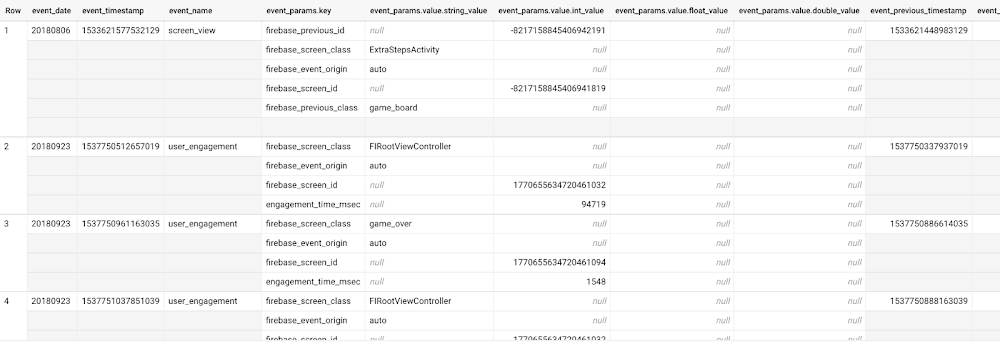
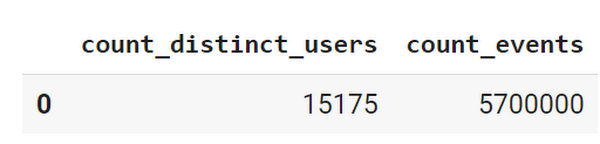
This dataset contains 5.7M events from over 15k users.
SELECTCOUNT(DISTINCT user_pseudo_id) as count_distinct_users,COUNT(event_timestamp) as count_eventsFROM`firebase-public-project.analytics_153293282.events_*
Our goal is to use BigQuery ML on the sample app dataset to predict propensity to user churn or not churn based on users’ demographics and activities within the first 24 hours of app installation.
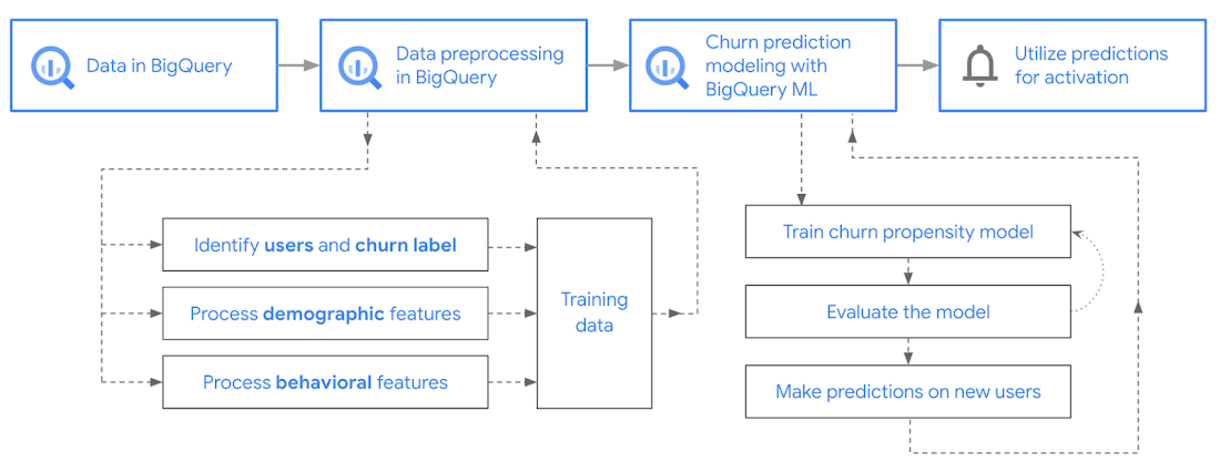
In the following sections, we’ll cover how to:
- Pre-process the raw event data from GA4
- Identify users & the label feature
- Process demographic features
- Process behavioral features
- Train classification model using BigQuery ML
- Evaluate the model using BigQueryML
- Make predictions using BigQuery ML
- Utilize predictions for activation
Pre-process the raw event data
You cannot simply use raw event data to train a machine learning model as it would not be in the right shape and format to use as training data. So in this section, we’ll go through how to pre-process the raw data into an appropriate format to use as training data for classification models.
This is what the training data should look like for our use case at the end of this section:
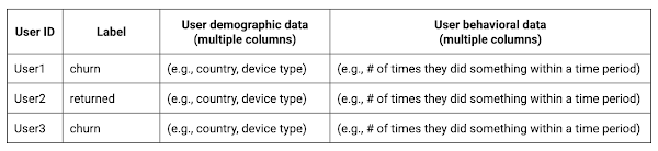
Notice that in this training data, each row represents a unique user with a distinct user ID (user_pseudo_id).
Identify users & the label feature
We first filtered the dataset to remove users who were unlikely to return the app anyway. We defined these ‘bounced’ users as ones who spent less than 10 mins with the app. Then we labeled all remaining users:
- churned: No event data for the user after 24 hours of first engaging with the app.
- returned: The user has at least one event record after 24 hours of first engaging with the app.
For your use case, you can have a different definition of bounce and churning. Also you can even try to predict something else other than churning, e.g.:
- whether a user is likely to spend money on in-game currency
- likelihood of completing n-number of game levels
- likelihood of spending n amount of time in-game etc.
In such cases, label each record accordingly so that whatever you are trying to predict can be identified from the label column.
From our dataset, we found that ~41% users (5,557) bounced. However, from the remaining users (8,031), ~23% (1,883) churned after 24 hours:
SELECTbounced,churned,COUNT(churned) as count_usersFROMbqmlga4.returningusersGROUP BY 1,2ORDER BY bounced
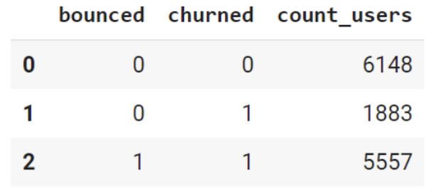
To create these bounced and churned columns, we used the following snippet of SQL code.
...#churned = 1 if last_touch within 24 hr of app installation, else 0IF (user_last_engagement < TIMESTAMP_ADD(user_first_engagement,INTERVAL 24 HOUR),1,0 ) AS churned,#bounced = 1 if last_touch within 10 min, else 0IF (user_last_engagement <= TIMESTAMP_ADD(user_first_engagement,INTERVAL 10 MINUTE),1,0 ) AS bounced,...
You can view the Jupyter Notebook for the full query used for materializing the bounced and churned labels.
Process demographic features
Next, we added features both for demographic data and for behavioral data spanning across multiple columns. Having a combination of both demographic data and behavioral data helps to create a more predictive model.
We used the following fields for each user as demographic features:
geo.countrydevice.operating_systemdevice.language
A user might have multiple unique values in these fields — for example if a user uses the app from two different devices. To simplify, we used the values from the very first user engagement event.
CREATE OR REPLACE VIEW bqmlga4.user_demographics AS (WITH first_values AS (SELECTuser_pseudo_id,geo.country as country,device.operating_system as operating_system,device.language as language,ROW_NUMBER() OVER (PARTITION BY user_pseudo_id ORDER BY event_timestamp DESC) AS row_numFROM `firebase-public-project.analytics_153293282.events_*`WHERE event_name="user_engagement")SELECT * EXCEPT (row_num)FROM first_valuesWHERE row_num = 1 #first engagement);
Process behavioral features
There is additional demographic information present in the GA4 export dataset, e.g. app_info, device, event_params, geo etc. You may also send demographic information to Google Analytics through each hit via user_properties. Furthermore, if you have first-party data on your own system, you can join that with the GA4 export data based on user_ids.
To extract user behavior from the data, we looked into the user’s activities within the first 24 hours of first user engagement. In addition to the events automatically collected by Google Analytics, there are also the recommended events for games that can be explored to analyze user behavior. For our use case, to predict user churn, we counted the number of times the follow events were collected for a user within 24 hours of first user engagement:
user_engagementlevel_start_quickplaylevel_end_quickplaylevel_complete_quickplaylevel_reset_quickplaypost_scorespend_virtual_currencyad_rewardchallenge_a_friendcompleted_5_levelsuse_extra_steps
The following query shows how these features were calculated:
WITHevents_first24hr AS (SELECTe.*FROM`firebase-public-project.analytics_153293282.events_*` eJOINbqmlga4.returningusers rONe.user_pseudo_id = r.user_pseudo_idWHERETIMESTAMP_MICROS(e.event_timestamp) <= r.ts_24hr_after_first_engagement)SELECTuser_pseudo_id,SUM(IF(event_name = 'user_engagement', 1, 0)) AS cnt_user_engagement,# ... repeated for all behavior data ...SUM(IF(event_name = 'use_extra_steps', 1, 0)) AS cnt_use_extra_steps,FROMevents_first24hrGROUP BY1
View the notebook for the query used to aggregate and extract the behavioral data. You can use different sets of events for your use case. To view the complete list of events, use the following query:
SELECTevent_name,COUNT(event_name) as event_countFROM`firebase-public-project.analytics_153293282.events_*`GROUP BY 1ORDER BYevent_count DESC
After this we combined the features to ensure our training dataset reflects the intended structure. We had the following columns in our table:
- User ID:
user_pseudo_id
- Label:
churned
- Demographic features
countrydevice_osdevice_language
- Behavioral features
cnt_user_engagementcnt_level_start_quickplaycnt_level_end_quickplaycnt_level_complete_quickplaycnt_level_reset_quickplaycnt_post_scorecnt_spend_virtual_currencycnt_ad_rewardcnt_challenge_a_friendcnt_completed_5_levelscnt_use_extra_stepsuser_first_engagement
At this point, the dataset was ready to train the classification machine learning model in BigQuery ML. Once trained, the model will output a propensity score between churn (churned=1) or return (churned=0) indicating the probability of a user churning based on the training data.
Train classification model
When using the CREATE MODEL statement, BigQuery ML automatically splits the data between training and test. Thus the model can be evaluated immediately after training (see the documentation for more information).
For the ML model, we can choose among the following classification algorithms where each type has its own pros and cons:
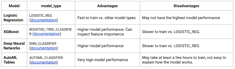
Often logistic regression is used as a starting point because it is the fastest to train. The query below shows how we trained the logistic regression classification models in BigQuery ML.
CREATE OR REPLACE MODEL bqmlga4.churn_logregTRANSFORM(EXTRACT(MONTH from user_first_engagement) as month,EXTRACT(DAYOFYEAR from user_first_engagement) as julianday,EXTRACT(DAYOFWEEK from user_first_engagement) as dayofweek,EXTRACT(HOUR from user_first_engagement) as hour,* EXCEPT(user_first_engagement, user_pseudo_id))OPTIONS(MODEL_TYPE="LOGISTIC_REG",INPUT_LABEL_COLS=["churned"]) ASSELECT*FROMbqmlga4.train
We extracted month, julianday, and dayofweek from datetimes/timestamps as one simple example of additional feature preprocessing before training. Using TRANSFORM() in your CREATE MODEL query allows the model to remember the extracted values. Thus, when making predictions using the model later on, these values won’t have to be extracted again. View the notebook for the example queries to train other types of models (XGBoost, deep neural network, AutoML Tables).
Evaluate model
Once the model finished training, we ran ML.EVALUATE to generate precision, recall, accuracy and f1_score for the model:
SELECT*FROMML.EVALUATE(MODEL bqmlga4.churn_logreg)

The optional THRESHOLD parameter can be used to modify the default classification threshold of 0.5. For more information on these metrics, you can read through the definitions on precision and recall, accuracy, f1-score, log_loss and roc_auc. Comparing the resulting evaluation metrics can help to decide among multiple models.Furthermore, we used a confusion matrix to inspect how well the model predicted the labels, compared to the actual labels. The confusion matrix is created using the default threshold of 0.5, which you may want to adjust to optimize for recall, precision, or a balance (more information here).
SELECTexpected_label,_0 AS predicted_0,_1 AS predicted_1FROMML.CONFUSION_MATRIX(MODEL bqmlga4.churn_logreg)
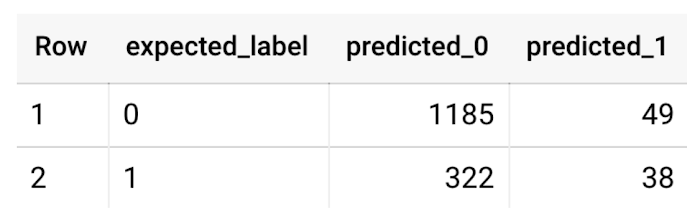
This table can be interpreted in the following way:

Make predictions using BigQuery ML
Once the ideal model was available, we ran ML.PREDICT to make predictions. For propensity modeling, the most important output is the probability of a behavior occurring. The following query returns the probability that the user will return after 24 hrs. The higher the probability and closer it is to 1, the more likely the user is predicted to return, and the closer it is to 0, the more likely the user is predicted to churn.
SELECTuser_pseudo_id,returned,predicted_returned,predicted_returned_probs[OFFSET(0)].prob as probability_returnedFROMML.PREDICT(MODEL bqmlga4.churn_logreg,(SELECT * FROM bqmlga4.train)) #can be replaced with a proper test dataset
Utilize predictions for activation
Once the model predictions are available for your users, you can activate this insight in different ways. In our analysis, we used user_pseudo_id as the user identifier. However, ideally, your app should send back the user_id from your app to Google Analytics. In addition to using first-party data for model predictions, this will also let you join back the predictions from the model into your own data.
- You can import the model predictions back into Google Analytics as a user attribute. This can be done using the Data Import feature for Google Analytics 4. Based on the prediction values you can Create and edit audiences and also do Audience targeting. For example, an audience can be users with prediction probability between 0.4 and 0.7, to represent users who are predicted to be “on the fence” between churning and returning.
- For Firebase Apps, you can use the Import segments feature. You can tailor user experience by targeting your identified users through Firebase services such as Remote Config, Cloud Messaging, and In-App Messaging. This will involve importing the segment data from BigQuery into Firebase. After that you can send notifications to the users, configure the app for them, or follow the user journeys across devices.
- Run targeted marketing campaigns via CRMs like Salesforce, e.g. send out reminder emails.
You can find all of the code used in this blogpost in the Github repository:
What’s next?
Continuous model evaluation and re-training
As you collect more data from your users, you may want to regularly evaluate your model on fresh data and re-train the model if you notice that the model quality is decaying.
Continuous evaluation—the process of ensuring a production machine learning model is still performing well on new data—is an essential part in any ML workflow. Performing continuous evaluation can help you catch model drift, a phenomenon that occurs when the data used to train your model no longer reflects the current environment.
To learn more about how to do continuous model evaluation and re-train models, you can read the blogpost: Continuous model evaluation with BigQuery ML, Stored Procedures, and Cloud Scheduler
More resources
If you’d like to learn more about any of the topics covered in this post, check out these resources:
- BigQuery export of Google Analytics data
- BigQuery ML quickstart
- Events automatically collected by Google Analytics 4
- Qwiklabs: Create ML models with BigQuery ML
Or learn more about how you can use BigQuery ML to easily build other machine learning solutions:
- How to build demand forecasting models with BigQuery ML
- How to build a recommendation system on e-commerce data using BigQuery ML
Let us know what you thought of this post, and if you have topics you’d like to see covered in the future! You can find us on Twitter at @polonglin and @_mkazi_.Thanks to reviewers: Abhishek Kashyap, Breen Baker, David Sabater Dinter.
How a Mid-Sized Firm is Shrinking Inventory Carryovers 50% with AI

7427
Of your peers have already read this article.
5:30 Minutes
The most insightful time you'll spend today!
For more than 10 years, NMK Textile Mills has manufactured bed linens for major retailers in the United States and Canada. As e-commerce exploded, the company’s co-founder saw an opportunity to grow the business. So, in addition to manufacturing bed linens wholesale for retail customers, NMK Textile Mills reworked its complete supply chain to manufacture products for California Design Den, which became an e-commerce retailer selling its own fashion-forward products directly to consumers online.
With California Design Den’s push into e-commerce, it became apparent the SMB company (with about 250 global employees) faced the same tough supply chain questions as large retail customers, including maintaining enough inventory to meet customer demand in a timely, efficient way.
California Design Den depended upon a myriad of systems to track its complex forecasting and reordering processes. Team members typically planned inventory manually using desktop spreadsheet software, which could lead to excess inventory. Accurately forecasting demand and supply was essential to the company’s financial success—but it was also a challenge.
A couple years ago, California Design Den partnered with Pluto7, a technology solutions provider that offers a software as a service (SaaS) called Planning In A Box. Leveraging Google Cloud Platform machine learning and artificial intelligence, Planning In A Box intelligently helps predict demand and balances it with supply.
But that was just the beginning. “Along the way, we realized that to compete with larger retailers, make quicker decisions, and move faster, we needed to go further,” says Deepak Mehrotra, Co-founder and Chief Adventurer at California Design Den.
With guidance from Pluto7, California Design Den began migrating its database to Google Cloud Platform. Using Google BigQuery, Google Compute Engine, Google Cloud SQL, and Google Cloud Storage, and experimenting with Google Cloud Vision and Google Cloud AutoML, the company is reducing inventory carryovers by more than 50%, improving the accuracy of demand planning quarter over quarter, and gaining granular insights into how individual SKUs are performing.
“We would need an army of data scientists to make faster decisions on pricing and inventory levels. With Google Cloud Platform machine learning and artificial intelligence, we don’t need that. We can make much faster pricing decisions to optimize profitability and move inventory.”
—Deepak Mehrotra, Co-founder and Chief Adventurer, California Design Den
No need for army of data scientists
“Using Google Cloud Platform machine learning and AI was essential for California Design Den if it was to compete successfully with larger retailers,” Deepak says.
For example, tastes and fashions in bed linens can change quickly and consumer prices fluctuate. With more than 2,500 SKUs, it wasn’t possible for California Design Den’s team to continuously monitor product demand and experiment with competitive pricing in real time.
“We would need an army of data scientists to make faster decisions on pricing and inventory levels,” says Deepak. “With Google Cloud Platform machine learning and artificial intelligence, we don’t need that. We can make much faster pricing decisions to optimize profitability and move inventory.”
By integrating all its data onto Google Cloud Platform, California Design Den’s team gains deeper insights into product sales over time, which in turn helps the company improve demand planning by better determining which styles to manufacture and sell in the future.
“When experienced employees leave, their knowledge leaves with them. By having all data in one place, and with machine learning and AI, California Design Den can go back in its history, look at products made or sold years ago, and analyze product performance.”
—Deepak Mehrotra, Co-founder and Chief Adventurer, California Design Den
Merging visuals with data
Before Google Cloud Platform, team members had to dig through spreadsheets and run scenarios to get a sense of how particular products had sold. The next step was to perform keyword searches across the company’s photo library in the cloud to find each product’s image. From there, a team member would insert the product images into a presentation, along with relevant data points, to provide a report for stakeholders on how particular styles performed.
Today, California Design Den, with the help of Pluto7, is integrating its entire product image library with its database on Google Cloud Platform. Experimenting with Google Cloud Vision and Google Cloud AutoML, California Design Den is moving towards a day when team members can run sales scenarios and get deep background data on individual product performance while viewing images of the relevant products.
Merging product visuals with data will help designers and team members better understand sales patterns over time and in context. In the past, making correlations between things like which sheet colors sold well in California, compared to how the same sheet colors performed on the East Coast, was something that California Design Den employees primarily did in their heads.
“When experienced employees leave, their knowledge goes with them,” says Manjunath Devadas, Founder and CEO at Pluto7. “By having all data in one place, and with machine learning and AI, California Design Den can go back in its history, look at products made or sold years ago, and analyze product performance.”
“We are literally growing the complexity of our business on all levels, including designing, manufacturing, selling, reordering, inventory holding—everything.”
—Deepak Mehrotra, Co-founder and Chief Adventurer, California Design Den
Reimagining supply-demand balancing
Pluto7’s mission statement is to democratize supply demand balancing with machine learning and AI. California Design Den is a case in point, as the combination of Planning In A Box and Google Cloud Platform gives the company greater control over its destiny.
“Big retailers used to tell us what to manufacture and how much they would pay for it,” says Deepak. “That was our primary business, and if we didn’t accept the terms, a competitor would.” Today, in addition to continuing to make products for retailers, California Design Den can design, make, and sell a variety of designs for itself, including custom and limited-edition products, thanks to Google Cloud Platform and Pluto7 software offerings. The payoff is not only in having a more diversified business. California Design Den also receives more favorable profit margins by selling its own products.
“We are literally growing the complexity of our business on all levels, including designing, manufacturing, selling, reordering, inventory holding—everything,” Deepak says. “We can make smaller batches. We can connect directly with consumers. We can identify the missing pieces—what should we produce next, when, and how much? We otherwise couldn’t afford the level of talent it would take to do this.”
Cutting through the noise
Google and Pluto7 software helped California Design Den reduce inventory carryovers by more than 50%. Inventory tracking and distribution, along with insights and visibility into product sales, are faster, more efficient, and accurate. Google Cloud Platform flexible pricing, speed, reliability, security, and scalability enable California Design Den to stay relevant and be more competitive.
In addition to benefiting from Google Cloud Platform, California Design Den relies on G Suite—also part of Google Cloud—to enhance collaboration among its global teams. Previously, the company’s email server would sometimes crash, due to the heavy load of sharing product photos and other data. “Gmail and Google Drive handle the everyday demands on the business effortlessly and reliably,” Deepak says.
“Google machine learning and AI enable us to cut through all the noise from raw data, so we can see what’s important. We can focus on analytics to guide us to success today and in the future.”
—Deepak Mehrotra, Co-founder and Chief Adventurer, California Design Den
The company is exploring additional ways to leverage Google Cloud Platform in the near future. For example, one possibility is to import customer reviews from sites where products are sold into Google BigQuery, and to use that data to perform sentiment analysis via Google Cloud Natural Language. It could provide another valuable data source to help California Design Den’s team decide where to focus future designs.
“Google machine learning and AI enable us to cut through all the noise from raw data, so we can see what’s important,” Deepak says. “We can focus on analytics to guide us to success today and in the future.”
Google’s Lesson on Leveraging AI and More to Optimize Cloud Value for Innovation
DOWNLOAD EXPLAINER4830
Of your peers have already downloaded this article
1:30 Minutes
The most insightful time you'll spend today!
Google has managed to stay ahead of the curve and demonstrate its ‘growth while staying innovative’ approach using advanced open technologies, AI/ML based analytics solutions, as well as tools for team collaboration and skill development, automation and storage security. Businesses too can achieve the same by deriving maximum value from its people and technology by following Google’s simple guide to stay innovative. Download to learn more.
How to Enhance Incremental Pipeline Performance while Ingesting Data into BigQuery

6307
Of your peers have already read this article.
3:00 Minutes
The most insightful time you'll spend today!
When you build a data warehouse, the important question is how to ingest data from the source system to the data warehouse. If the table is small you can fully reload a table on a regular basis, however, if the table is large a common technique is to perform incremental table updates. This post demonstrates how you can enhance incremental pipeline performance when you ingest data into BigQuery.
Setting up a standard incremental data ingestion pipeline
We will use the below example to illustrate a common ingestion pipeline that incrementally updates a data warehouse table. Let’s say that you ingest data into BigQuery from a large and frequently updated table in the source system, and you have Staging and Reporting areas (datasets) in BigQuery.

The Reporting area in BigQuery stores the most recent, full data that has been ingested from the source system tables. Usually you create the base table as a full snapshot of the source system table. In our running example, we use BigQuery public data as the source system and create reporting.base_table as shown below. In our example each row is identified by a unique key which consists of two columns: block_hash and log_index.
CREATE TABLE reporting.base_table --156 GB processedPARTITION BY TIMESTAMP_TRUNC(block_timestamp, DAY) ASSELECT log_index, data, topics, block_timestamp, block_hashFROM bigquery-public-data.crypto_ethereum.logsWHERE block_timestamp BETWEEN TIMESTAMP '2020-01-01' AND TIMESTAMP '2020-11-30';
In data warehouses it is common to partition a large base table by a datetime column that has a business meaning. For example, it may be a transaction timestamp, or datetime when some business event happened, etc. The idea is that data analysts who use the data warehouse usually need to analyze only some range of dates and rarely need the full data. In our example, we partition the base table by block_timestamp which comes from the source system.
After ingesting the initial snapshot you need to capture changes that happen in the source system table and update the reporting base table accordingly. This is when the Staging area comes into the picture. The staging table will contain captured data changes that you will merge into the base table. Let’s say that in our source system on a regular basis we have a set of new rows and also some updated records. In our example we mock the staging data as follows: first, we create new data, than we mock the updated records:
CREATE TABLE staging.load_delta AS --5 GB processedSELECT log_index, data, topics, block_timestamp, block_hashFROM bigquery-public-data.crypto_ethereum.logsWHERE block_timestamp BETWEEN TIMESTAMP '2020-12-01' AND TIMESTAMP '2020-12-07';INSERT INTO staging.load_delta --2 GB processedSELECT log_index, CONCAT(data, RAND()), topics, block_timestamp, block_hashFROM bigquery-public-data.crypto_ethereum.logs TABLESAMPLE SYSTEM (5 PERCENT)WHERE block_timestamp BETWEEN TIMESTAMP '2020-10-01' AND TIMESTAMP '2020-11-30';
Next, the pipeline merges the staging data into the base table. It joins two tables by unique key and than updates the changed value or inserts a new row
MERGE INTO reporting.base_table T --161 GB processedUSING staging.load_delta SON T.block_hash = S.block_hashAND T.log_index = S.log_indexWHEN MATCHED THEN UPDATE SETT.data = S.dataWHEN NOT MATCHED THEN INSERT (log_index, data, topics, block_timestamp, block_hash)VALUES (log_index, data, topics, block_timestamp, block_hash);
It is often the case that the staging table contains keys from various partitions but the number of those partitions are relatively small. It holds, for instance, because in the source system the recently added data may get changed due to some initial errors or ongoing processes but older records are rarely updated. However, when the above MERGE gets executed, BigQuery scans all partitions in the base table and processes 161 GB of data. You might add additional join condition on block_timestamp:
MERGE INTO reporting.base_table T --161 GB processedUSING staging.load_delta SON T.block_hash = S.block_hashAND T.log_index = S.log_indexAND T.block_timestamp = S.block_timestampWHEN MATCHED THEN UPDATE SETT.data = S.dataWHEN NOT MATCHED THEN INSERT (log_index, data, topics, block_timestamp, block_hash)VALUES (log_index, data, topics, block_timestamp, block_hash);
But BigQuery would still scan all partitions in the base table because condition T.block_timestamp = S.block_timestamp is a dynamic predicate and BigQuery doesn’t automatically push such predicates down from one table to another in MERGE.
Can you improve the MERGE efficiency by making it scan less data? The answer is Yes.
As described in the MERGE documentation, pruning conditions may be located in a subquery filter, a merge_condition filter, or a search_condition filter. In this post we show how you can leverage the first two. The main idea is to turn a dynamic predicate into a static predicate.
Steps to enhance your ingestion pipeline
The initial step is to compute the range of partitions that will be updated during the MERGE and store it in a variable. As was mentioned above, in data ingestion pipelines, staging tables are usually small so the cost of the computation is relatively low.
DECLARE src_range STRUCT<date_min TIMESTAMP, date_max TIMESTAMP> --115 MB processedDEFAULT(SELECT STRUCT(MIN(block_timestamp) AS date_min,MAX(block_timestamp) AS date_max) FROM staging.load_delta);
Based on your existing ETL/ELT pipeline, you can add the above code as-is to your pipeline or you can compute date_min, data_max as part of some already existing transformation step. Alternatively, date_min, data_max can be computed on the Source System side while capturing the next ingestion data batch.
After computing date_min, date_max you pass those values to the MERGE statement as static predicates. There are several ways to enhance the MERGE and prune partitions in the base table based on precomputed date_min, data_max.
If your initial MERGE statement uses a subquery, you can incorporate a new filter into it:
BEGINDECLARE src_range STRUCT<date_min TIMESTAMP, date_max TIMESTAMP> --115 MB processedDEFAULT(SELECT STRUCT(MIN(block_timestamp) AS date_min,MAX(block_timestamp) AS date_max) FROM staging.load_delta);MERGE INTO reporting.base_table T --41 GB processedUSING (SELECT *FROM staging.load_deltaWHERE block_timestamp BETWEEN src_range.date_min AND src_range.date_max) SON T.block_hash = S.block_hashAND T.log_index = S.log_indexAND T.block_timestamp = S.block_timestampWHEN MATCHED THEN UPDATE SETT.data = S.dataWHEN NOT MATCHED THEN INSERT (log_index, data, topics, block_timestamp, block_hash)VALUES (log_index, data, topics, block_timestamp, block_hash);END;
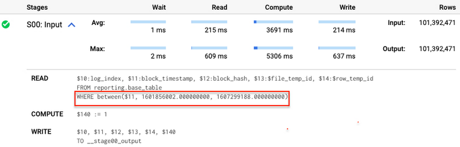
Note that you add the static filter to the staging table and keep T.block_timestamp = S.block_timestamp to convey to BigQuery that it can push that filter to the base table. This MERGE processes 41 GB of data in contrast to the initial 161 GB. You can see in the query plan that BigQuery pushes the partition filter from the staging table to the base table:
This type of optimization, when a pruning condition is pushed from a subquery to a large partitioned or clustered table, is not unique for MERGE. It also works for other types of queries. For instance:
SELECT * -- 41 GB processedFROM reporting.base_table TINNER JOIN staging.load_delta SON T.block_hash = S.block_hashAND T.log_index = S.log_indexAND T.block_timestamp = S.block_timestampWHERE S.block_timestamp BETWEEN TIMESTAMP '2020-10-05' AND TIMESTAMP '2020-12-07'
And you can check the query plan to verify that BigQuery pushed down the partition filter from one table to another.
Moreover, for SELECT statements, BigQuery can automatically infer a filter predicate on a join column and push it down from one table to another if your query meets the following criteria:
- The target table must be clustered or partitioned.
- The result size of the other table, i.e. after applying all filters, must qualify for broadcast join. Namly, the result set must be relatively small, less than ~100MB.
In our running example, reporting.base_table is partitioned by block_timestamp. If you define a selective filter on staging.load_delta and join two tables, you can see an inferred filter on the join key pushed to the target table
SELECT *FROM reporting.base_table TINNER JOIN staging.load_delta SON T.block_timestamp = S.block_timestampWHERE S.block_hash = '0x0c1caa16b34d94843aabfebc0d5a961db358135988f7498a6fdc450ad55f0870'
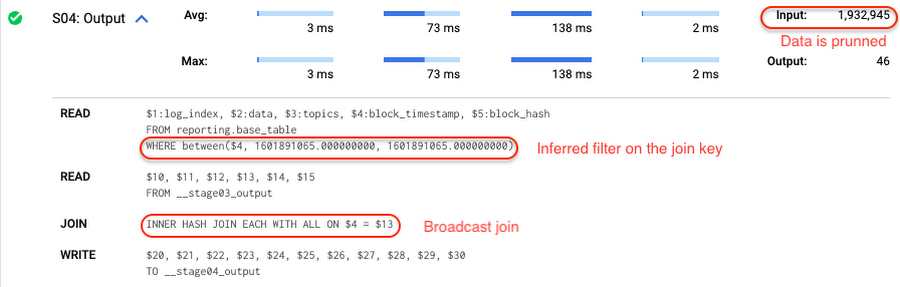
There is no requirement to join tables by partitioning or clustering key to kick off this type of optimization. However, in this case the pruning effect on the target table would be less significant.
But let us get back to the pipeline optimizations. Another way to enhance MERGE is to modify the merge_condition filter by adding static predicate on the base table:
BEGINDECLARE src_range STRUCT<date_min TIMESTAMP, date_max TIMESTAMP> --115 MB processedDEFAULT(SELECT STRUCT(MIN(block_timestamp) AS date_min,MAX(block_timestamp) AS date_max) FROM staging.load_delta);MERGE INTO reporting.base_table T --41 GB processedUSING staging.load_delta SON T.block_hash = S.block_hashAND T.log_index = S.log_indexAND T.block_timestamp BETWEEN src_range.date_min AND src_range.date_maxWHEN MATCHED THEN UPDATE SETT.data = S.dataWHEN NOT MATCHED THEN INSERT (log_index, data, topics, block_timestamp, block_hash)VALUES (log_index, data, topics, block_timestamp, block_hash);END;
To summarize, here are the steps that you can perform to enhance incremental ingestion pipelines in BigQuery. First you compute the range of updated partitions based on the small staging table. Next, you tweak the MERGE statement a bit to let BigQuery know to prune data in the base table.
All the enhanced MERGE statements scanned 41 GB of data, and setting up the src_range variable took 115 MB. Compare it with the initial 161 GB scan. Moreover, given that computing src_range may be incorporated into some existing transformation in your ETL/ELT, it results in a good performance improvement which you can leverage in your pipelines.
In this post we described how to enhance data ingestion pipelines by turning dynamic filter predicates into static predicates and letting BiQuery prune data for us. You can find more tips on BigQuery DML tuning here.
Special thanks to Daniel De Leo, who helped with examples and provided valuable feedback on this content.
More Relevant Stories for Your Company




How adidas’s Marketing Team Benefits from Google Cloud Marketing Platform
We live in a world where the consumer journey is no longer linear, making it difficult to know when to deliver a brand message or a product message. “We talk a lot about the consumer journey no longer being linear. It’s very difficult to know when the consumer is going


Metro Consolidates 100 SAP Instances on Google Cloud
German retailer Metro, with operations in 25 countries across Europe and Asia and employing over 150,000 people, decided to consolidate its 100 SAP instances into one SAP S/4HANA system running on the Google Cloud Platform. This helped the company lower costs, increase efficiency, and improve customer experience. In addition, the



90-Sec Demos of Truly Incredible Customer Care Calls Powered By AI
How real, fast, and easy do you think an AI-powered call center experience is for customers today? It's likely you have seen AI-powered chatbots and are deeply unimpressed with the static nature of the interaction between customers and service representatives. But that's not how Google Cloud's AI-powered contact centers are.



Breakthrough Insights Across the Life Sciences Value Chain
New science and patient centricity require increasing reliance on data and deeper insights. Accenture’s life sciences customers have been demanding answers to this need, and want a solution with an open platform. Enter INTIENT, Accenture’s life sciences platform that is powered by Google Cloud. INTIENT generates insights throughout the life
