





Optimizing Terabyte-scale PostgreSQL Migrations to Cloud SQL Using Searce

3028
Of your peers have already read this article.
2:30 Minutes
The most insightful time you'll spend today!
Google Cloud allows you to move your PostgreSQL databases to Cloud SQL with Database Migration Service (DMS). DMS gives you the ability to replicate data continuously to the destination database, while the source is live in production, enabling you to migrate with minimum downtime.
However, terabyte-scale migrations can be complex. For instance, if your PostgreSQL database has Large Objects, then you will require some downtime to migrate them manually as that is a limitation of DMS. There are few more such limitations – check out known limitations of DMS. If not handled carefully, these steps can extend the downtime during cutover, lead to performance impact on the source instance, or even delay the project delivery date. All this may mean significant business impact.
Searce is a technology consulting company, specializing in modernizing application and database infrastructure by leveraging cloud, data and AI. We empower our clients to accelerate towards the future of their business. In our journey, we have helped dozens of clients migrate to Cloud SQL, and have found terabyte-scale migrations to be the toughest for the reasons mentioned earlier.
This blog centers around our work in supporting an enterprise client whose objective was to migrate dozens of terabyte scale, mission-critical PostgreSQL databases to Cloud SQL with minimum downtime. Their largest database was 20TB in size and all the databases had tables with large objects and some tables did not have primary keys. Note that DMS had a limitation of not supporting migration of tables without a primary key during the time of this project. In June 2022, DMS released an enhancement to support the migration of tables without a primary key.
In this blog, we share with you our learnings about how we simplified and optimized this migration, so that you can incorporate our best practices into your own migrations. We explore mechanisms to reduce the downtime required for operations not handled by DMS by ~98% with the use of automation scripts. We also explore database flags in PostgreSQL to optimize DMS performance and minimize the overall migration time by ~15%.
Optimize DMS performance with database flags
Once the customer made the decision to migrate PostgreSQL databases to Google Cloud SQL, we considered two key factors that would decide business impact – migration effort and migration time. To minimize effort for the migration of PostgreSQL databases, we leveraged Google Cloud’s DMS (Database Migration Service) as it is very easy to use and it does the heavy lifting by continuously replicating data from the source database to the destination Cloud SQL instance, while the source database is live in production.
How about migration time? For a terabyte-scale database, depending on the database structure, migration time can be considerably longer. Historically, we observed that DMS took around 3 hours to migrate a 1 TB database. In other cases, where the customer database structure was more complex, migration took longer. Thankfully, DMS takes care of this replication while the source database is live in production, so no downtime is required during this time. Nevertheless, our client would have to bear the cost of both the source and destination databases which for large databases, might be substantial. Meanwhile, if the database size increased, then replication could take even longer, increasing the risk of missing the customer’s maintenance window for the downtime incurred during cutover operations. Since the customer’s maintenance window was monthly, we would have to wait for 30 more days for the next maintenance window, requiring the customer to bear the cost of both the databases for another 30 days. Furthermore, from a risk management standpoint, the longer the migration timeframe, the greater the risk that something could go wrong. Hence, we started exploring options to reduce the migration time. Even the slightest reduction in migration time could significantly reduce the cost and risk.
We explored options around tuning PostgreSQL’s database flags on the source database. While DMS has its own set of prerequisite flags for the source instance and database, we also found that flags like shared_buffers, wal_buffers and maintenance_work_mem helped accelerate the replication process through DMS. These flags needed to be set to a specific value to get the maximum benefit out of each of them. Once set, their cumulative impact was a reduction in time for DMS to replicate a 1 TB database by 4 hours, that is, reduction of 3.5 days for a 20 TB database. Let’s dive into each of them.
Shared Buffers
PostgreSQL uses two buffers – its own internal buffer and the kernel buffered IO. In other words, that data is stored in memory twice. The internal buffer is called shared_buffers, and it determines the amount of memory used by the database for the operating system cache. By default this value is set conservatively low. However, increasing this value on the source database to fit our use case helped increase the performance of read heavy operations, which is exactly what DMS does once a job has been initialized.
After multiple iterations, we found that if the value was set to 55% of the database instance RAM, it boosted the replication performance (a read heavy operation) by a considerable amount and in turn reduced the time required to replicate the data.
WAL Buffers
PostgreSQL relies on Write-Ahead Logging (WAL) to ensure data integrity. WAL records are written to buffers and then flushed to disk. The flag wal_buffers, determines the amount of shared memory used for WAL data that has not yet been written to disk – records that are yet to be flushed. We found that increasing the value for wal_buffers from the default value of 16MB to about 3% of the database instance’s RAM significantly improved the write performance by writing fewer but larger files to the disk at each transaction commit.
Maintenance Work Mem
PostgreSQL maintenance operations, such as VACUUM, CREATE INDEX, and ALTER TABLE ADD FOREIGN KEY, consume their own specific memory. This memory is referred to as maintenance_work_mem. Unlike other operations, PostgreSQL maintenance operations can only be performed sequentially by the database. Setting a value significantly higher than the default value of 64 MB meant that no maintenance operation would block the DMS job. We found that maintenance_work_mem worked best at the value of 1 GB.
Resize source instance to avoid performance impact
Each of these three flags tune how PostgreSQL utilizes memory resources. Hence, it was imperative that before setting these flags, we needed to upsize the source database instance to accommodate them. Without upsizing the database instances, we could have caused application performance degradation, as more than half of the total database memory would be allocated to the processes managed by these flags.
We calculated the memory required by the flags mentioned above, and found that each flag needed to be set to a specific percentage of the source instance’s memory, irrespective of the existing values that might be set for the flags:
- shared_buffers: 55% of source instance’s memory
- wal_buffers: 3% of source instance’s memory
- maintenance_work_mem: 1 GB
We added the individual memory requirements by the flags, and found that 58% of the RAM at least will be taken up by these memory flags. For example, if a source instance used 100GB of memory, 58GB would be taken up by shared_buffers and wal_buffers, and an additional 1GB by maintenance_work_mem. As the original value of these flags was very low (~200MB), we upsized the RAM of the source database instance by 60% in order to ensure that the migration did not impact source performance on the application live in production.
Avoid connection error with WAL sender timeout flag
While using Google Cloud’s DMS, if the connection is terminated between DMS and the Cloud SQL instance during the ‘Full Dump in Progress’ phase of the DMS job, the DMS job fails and needs to be reinitiated. Encountering timeouts, especially while migrating a terabyte-scale database, would mean multiple days’ worth of migration being lost and a delay in the cutover plan. For example, if the connection of the DMS job for a 20TB database migration is lost after 10 days, the DMS job will have to be restarted from the beginning, leading to 10 days’ worth of migration effort being lost.
Adjusting the WAL sender timeout flag (wal_sender_timeout) helped us avoid terminating replication connections that were inactive for a long time during the full dump phase. The default value for this flag is 60 seconds. To avoid these connections from terminating, and to avoid such high impact failures, we set the value of this flag to 0 for the duration of database migration. This would avoid connections getting terminated and allowed for smoother replication through the DMS jobs.
Generally, for all the database flags we talked about here, we advised our customer to restore the default flag values once the migration completed.
Reduce downtime required for DMS limitations by automation
While DMS does the majority of database migration through continuous replication when the source database instance is live in production, DMS has certain migration limitations that cannot be addressed when the database is live. For PostgreSQL, the known limitations of DMS include:
- Any new tables created on the source PostgreSQL database after the DMS job has been initialized are not replicated to the destination PostgreSQL database.
- Tables without primary keys on the source PostgreSQL database are not migrated. For those tables, DMS migrated only the schema. This is no longer a limitation after the June 2022 product update.
- The large object (LOB) data type is not supported by DMS.
- Only the schema for Materialized Views is migrated; the data is not migrated.
- All data migrated is created under the ownership of cloudsqlexternalsync.
We had to address these aspects of the database migration manually. Since our client’s database had data with the large object data type, tables without primary keys, and frequently changing table structures that cannot be migrated by DMS, we had to manually export and import that data after DMS did most of the rest of the data migration. This part of database migration required downtime to avoid data loss. For a terabyte-scale database, this data can be in the hundreds of GBs, which means higher migration time and hence higher downtime. Furthermore, when you have dozens of databases to migrate, it can be stressful and error-prone for a human to perform these operations while on the clock during the cutover window!
This is where automation helped save the day! Automating the migration operations during the downtime period not only reduced the manual effort and error risk, but also provided a scalable solution that could be leveraged for the migration of 100s of PostgreSQL database instances to Cloud SQL. Furthermore, by leveraging multiprocessing and multithreading, we were able to reduce the total migration downtime for 100s of GBs of data by 98%, thereby reducing the business impact for our client.
How do we get there?
We laid out all the steps that need to be executed during the downtime – that is, after the DMS job has completed its replication from source to destination and before cutting over the application to the migrated database. You can see a chart mapping out the sequence of operations that are performed during the downtime period in Fig 1.
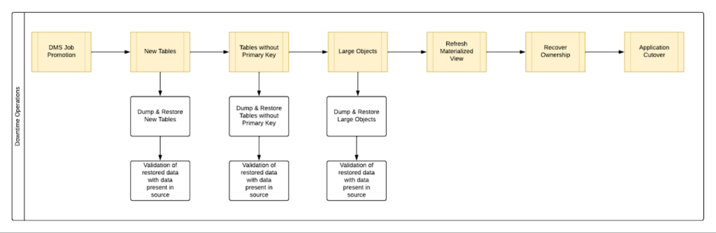
By automating all the downtime operations in this sequential approach, we observed that it took 13 hours for the entire downtime flow to execute for a 1 TB database. This included the migration of 250 MB in new tables, 60 GB in tables without primary keys and 150 GB in large objects.
One key observation we made was that, out of all the steps, only three steps took most of the time: migrating new tables, migrating tables without primary keys, and migrating large objects. These took the longest time because they all required dump and restore operations for their respective tables. However, these three steps did not have a hard dependency on each other as they individually targeted different tables. So we tried to run them in parallel as you can see in Fig 2. But the steps following them – ‘Refresh Materialized View’ and ‘Recover Ownership’ – had to be performed sequentially as they targeted the entire database.
However, running these three steps in parallel required upsizing the Cloud SQL instances, as we wanted to have sufficient resources available for each step. This led us to increase the Cloud SQL instances’ vCPU by 50% and memory by 40%, since the export and import operations depended heavily on vCPU consumption as opposed to memory consumption.
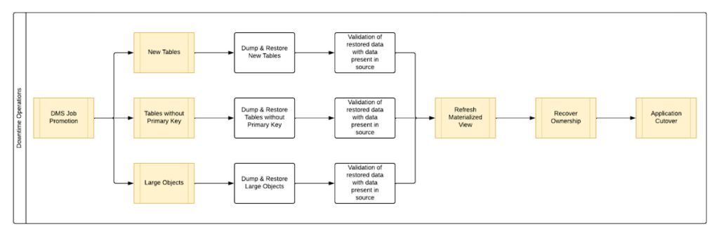
Migrating the new tables (created after the DMS job was initiated) and tables without primary keys was straightforward as we were able to leverage the native utilities offered by PostgreSQL – pg_dump and pg_restore. Both utilities process tables in parallel by using multiple threads– the higher the table count, the higher the number of threads that could be executed in parallel, allowing faster migration. With this revised approach, for the same 1 TB database, it still took 12.5 hours for the entire downtime flow to execute.
This improvement reduced the cutover downtime, but we still found that we needed a 12.5 hour window to complete all the steps. We then discovered that 99% of the time of downtime was taken up by just one step: exporting and importing 150 GB of large objects. It turned out that multiple threads could not be used to accelerate the dump and restore large objects in PostgreSQL. Hence, migrating the large objects single handedly extended the downtime for migration by hours. Fortunately, we were able to come up with a workaround for that.
Optimize migration of Large Object from PostgreSQL database
PostgreSQL contains a large objects facility that provides stream-style access to data stored in a special large-object structure. When large objects are stored, they are broken down into multiple chunks and stored in different rows of the database, but are connected under a single Object Identifier (OID). This OID can thus be used to access any stored Large Object. Although users can add large objects to any table in the database, under the hood, PostgreSQL physically stores all large objects within a database in a single table called pg_largeobjects.
While leveraging pg_dump and pg_restore for export and import of large objects, this single table – pg_largeobject, becomes a bottleneck as the PostgreSQL utilities cannot execute multiple threads for parallel processing, since it’s just one table. Typically, the order of operations for these utilities looks something like this:
- pg_dump reads the data to be exported from the source database
- pg_dump writes that data into the memory of the client where pg_dump is being executed
- pg_dump writes from memory to the disk of the the client (a second write operation)
- pg_restore reads the data from the client’s disk
- pg_restore writes the data to the destination database
Normally, these utilities would need to be executed sequentially to avoid data loss or data corruption due to conflicting processes. This leads to further increase in migration time for large objects.
Our workaround for this single-threaded process involved two elements. First, with our solution, we eliminated the second write operation – write from memory to disk (point #3). Instead, once the data was read and written into memory, our program would begin the import process and write data to the destination database. Second, since pg_dump and pg_restore could not use multiple threads to process the large objects in just the pg_largeobjects table, we took it upon ourselves to develop a solution that could use multiple threads. The thread count was based on the number of OIDs in the table – pg_largeobjects, and break that single table into smaller chunks for parallel execution.
This approach brought down Large Object migration operation from hours to minutes, therefore bringing down the downtime needed for all operations to be completed that DMS cannot handle, for the same 1 TB database, from 13 hours to just 18 minutes. A reduction of ~98% in the required downtime.
Conclusion
After multiple optimizations and dry runs, we were able to develop a procedure for our client to migrate dozens of terabyte-scale PostgreSQL databases to Google Cloud SQL with a minimal business impact. We developed practices to optimize DMS-based migration by 15% using database flags and reduce downtime by 98% with the help of automation and innovation. These practices can be leveraged for any terabyte-scale migration of PostgreSQL databases to Google Cloud SQL to accelerate migration, minimize downtime and avoid performance impact on mission critical applications.
6078
Of your peers have already watched this video.
1:30 Minutes
The most insightful time you'll spend today!
Explore the Innovations and Architecture Powering Spanner and BigQuery
Previously, databases had architectures with tightly coupled storage and compute. This resulted in higher latency, and with faster networks these constraints no longer surface. With Google Cloud’s BigQuery and CloudSpanner, the storage and compute architecture have been separated, allowing for better scalability and availability to address businesses’ high throughput data needs.
Watch the video to understand how these database and analysis products leverage Google’s distributed storage system, in-house custom network hardware and software, internal cluster management system and more!
Make Meaningful Analysis with Geo Boundary Public Datasets on BigQuery

6340
Of your peers have already read this article.
4:00 Minutes
The most insightful time you'll spend today!
Geospatial data is a critical component for a comprehensive analytics strategy. Whether you are trying to visualize data using geospatial parameters or do deeper analysis or modeling on customer distribution or proximity, most organizations have some type of geospatial data they would like to use – whether it be customer zipcodes, store locations, or shipping addresses. However, converting geographic data into the correct format for analysis and aggregation at different levels can be difficult. In this post, we’ll walk through some examples of how you can leverage the Google Cloud platform alongside Google Cloud Public Datasets to perform robust analytics on geographic data. The full queries can be accessed from this notebook here.
Public US Geo Boundaries dataset
BigQuery hosts a slew of public datasets for you to access and integrate into your analytics. Google pays for the storage of these datasets and provides public access to the data via the bigquery-public-data project. You only pay for queries against the data. Plus, the first 1 TB per month is free! These public datasets are valuable on their own, but when joined against your own data they can unlock new analytics use cases and save the team a lot of time.
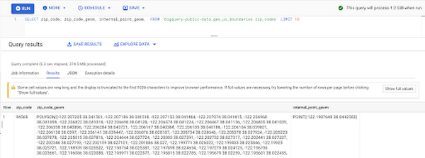
Within the Google Cloud Public Datasets Program there are several geographic datasets. Here, we’ll work with the geo_us_boundaries dataset, which contains a set of tables that have the boundaries of different geospatial areas as polygons and coordinates based on the center point (GEOGRAPHY column type in BigQuery), published by the US Census Bureau.
Mapping geospatial points to hierarchical areas
Many times you will find yourself in situations where you have a string representing an address. However, most tools require lat/long coordinates to actually plot points. Using the Google Maps Geocoding API we can convert an address into a lat/long and then store the results in the BigQuery table.
With a lat/long representation of our point, we can join our initial dataset back onto any of the tables here using the ST_WITHIN function. This allows us to check and see if a point is within the specified polygon.
ST_WITHIN(geography_1, geography_2)
This can be helpful for ensuring standard nomenclature; for example, metropolitan areas that might be named differently. The query below maps each customers’ address to a given metropolitan area name.
SELECTcust.id as customer_id,metro.name as metro_nameFROM `looker-private-demo.retail.customers` as cust,`bigquery-public-data.geo_us_boundaries.metropolitan_divisions` as metroWHERE ST_WITHIN(ST_GEOGPOINT(cust.longitude, cust.latitude),metro.metdiv_geom)
It can also be useful for converting to designated market area (DMA), which is often used in creating targeted digital marketing campaigns.
SELECTcust.id as customer_id,dma.dma_nameFROM `looker-private-demo.retail.customers` as cust,`bigquery-public-data.geo_us_boundaries.designated_market_area` as dmaWHERE ST_WITHIN(ST_GEOGPOINT(cust.longitude, cust.latitude),dma.dma_geom)
Or for filling in missing information; for example, some addresses may be missing zip code which results in incorrect calculations when aggregating up to the zipcode level. By joining onto the zip_codes table we can ensure all coordinates are mapped appropriately and aggregate up from there.
SELECTzip.zip_code,count(distinct cust.id) as unique_customersFROM `looker-private-demo.retail.customers` as cust,`bigquery-public-data.geo_us_boundaries.zip_codes` as zipWHERE ST_WITHIN(ST_GEOGPOINT(cust.longitude, cust.latitude),zip.zip_code_geom)GROUP BY 1
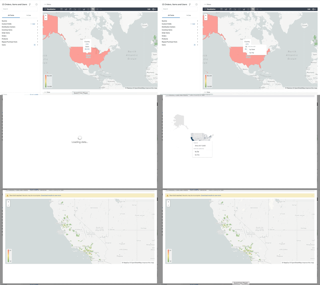
Note that the zip code table isn’t a comprehensive list of all US zip codes, they are zip code tabulation areas (ZCTAs). Details about the differences can be found here. Additionally, the zip code table gives us hierarchical information, which allows us to perform more meaningful analytics. One example is leveraging hierarchical drilling in Looker. I can aggregate my total sales up to the country level, and then drill down to state, city and zipcode to identify where sales are highest. You can also use the BigQuery GeoViz tool to visualize geospatial data!
Aside from simply checking if a point is within an area, we can also use ST_DISTANCE to do something like find the closest city using the centerpoint for the metropolitan area table.
SELECTcust.id as customer_id,ARRAY_AGG(metro.name order by ST_DISTANCE(ST_GEOGPOINT(cust.longitude, cust.latitude),metro.internal_point_geom) asc limit 1)[offset(0)] as metro_nameFROM`looker-private-demo.retail.customers` as cust,`bigquery-public-data.geo_us_boundaries.metropolitan_divisions` as metroGROUP BY cust.id
This concept doesn’t just hold true for points, we can also leverage other GIS functions to see if a geospatial area is contained within areas that are listed in the boundaries datasets. If your data comes into BigQuery as a GeoJSON string, we can convert it to a GEOGRAPHY type using the ST_GEOGFROMGEOJSON function. Once our data is in a GEOGRAPHY type we can do things like check to see what urban area the geo is within – using either ST_WITHIN or ST_INTERSECTS to account for partial coverage. Here, I am using the customer’s zip code to find all metropolitan divisions where the zip code polygon and the metropolitan polygon intersect. I am then selecting the metropolitan area that has the most overlap (or the intersection has the largest area) to be the customer’s metro that we use for reporting.
SELECTcust.id as customer_id,ARRAY_AGG(metro.name order by ST_AREA(ST_INTERSECTION(zip.zip_code_geom,metro.metdiv_geom)) desc limit 1)[offset(0)] as metro_nameFROM`looker-private-demo.retail.customers` as custJOIN `bigquery-public-data.geo_us_boundaries.zip_codes` as zip on cust.zip=zip.zip_code,`bigquery-public-data.geo_us_boundaries.metropolitan_divisions` as metroWHERE ST_INTERSECTS(zip.zip_code_geom,metro.metdiv_geom)GROUP BY cust.id
The same ideas can be applied to the other tables in the dataset including the county, urban areas and National Weather Service forecast regions (which can also be useful if you want to join your datasets onto weather data).
Correcting for data discrepancy
One problem that we may run into when working with geospatial data is that different data sources may have different representations of the same information. For example, you might have one system that records state as a two letter abbreviation and another using the full name. Here, we can use the state table to join the different datasets.
SELECTst.state_name,sum(ab.sales+fn.sales) as total_salesFROM `bigquery-public-data.geo_us_boundaries.states` as stLEFT JOIN abbreviated_table as ab on ab.state = st.stateLEFT JOIN fullname_table as fn on fn.state = st.state_nameWHERE COALESCE(ab.state, fn.state) IS NOT NULLGROUP BY 1
Another example might be using the tables as a source of truth for fuzzy matching. If the address is a manually entered field somewhere in your application, there is a good chance that things will be misspelled. Different representations of the same name may prevent tables from joining with each other or lead to duplicate entries when performing aggregations. Here, I use a simple Soundex algorithm to generate a code for each county name, using helper functions from this blog post. We can see that even though some are misspelled they have the same Soundex code.
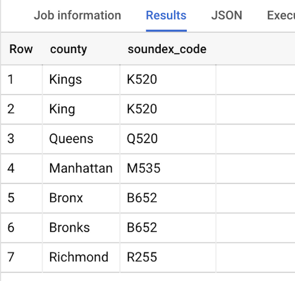
Next, we can join back onto our counties table so we make sure to use the correct spelling of the county name. Then, we can simply aggregate our data for more accurate reporting.
SELECTc.county_name,sum(sales) as total_salesFROMtableJOIN `bigquery-public-data.geo_us_boundaries.counties` as con testing.dq_fm_Soundex(table.county) = testing.dq_fm_Soundex(c.county_name)WHERE c.state_fips_code = cast(36 as string)GROUP BY 1
Note that fuzzy matching definitely isn’t perfect and you might need to try different methods or apply certain filters for it to work best depending on the specifics of your data.
The US Geo Boundary datasets allow you to perform meaningful geographic analysis without needing to worry about extracting, transforming or loading additional datasets into BigQuery. These datasets, along with all the other Google Cloud Public Datasets, will be available in the Analytics Hub. Please sign up for the Analytics Hub preview, which is scheduled to be available in the third quarter of 2021, by going to g.co/cloud/analytics-hub.
How We Built a Brand New Bank on Google Cloud and Cloud Spanner: The First Scalable, Enterprise-grade, Database Service
6556
Of your peers have already read this article.
6:30 Minutes
The most insightful time you'll spend today!
Editor’s note: Technology today lets companies of any size take on entire industries simply with an innovative business model plus digital distribution. Take Shine, a French startup whose platform helps freelancers manage their finances — and their administrative commitments. Here, Raphael Simon, Shine’s CTO and co-founder, talks about why Shine built a new bank on Google Cloud Platform, and in particular Cloud Spanner.
More and more people are deciding to take the plunge and start a freelance career. Some of them by choice, others out of necessity. One of their biggest pain points is dealing with administrative tasks.
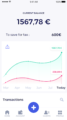
In some countries, especially in Europe, the administrative burden of being a freelancer is similar to what a company of 10 or more people deals with. A freelancer doesn’t necessarily have the time or skills to manage all this paperwork. So we are building a new bank for freelancers from the ground up that helps automate administrative tasks associated with their business.
Shine’s banking services and financial tools make it as easy to work as a freelancer as it is to work for a larger company. We deal with administrative tasks on behalf of the freelancer so that he or she can focus on their job: finding and wowing clients.

Building our infrastructure
As a new bank, we had the opportunity to build our infrastructure from the ground up. Designing an infrastructure and choosing a database presents tough decisions, especially in the financial services world. Financial institutions come under tremendous scrutiny to demonstrate stability and security. Even a tiny leak of banking data can have tremendous consequences both for the bank and its clients, and any service interruption can trigger a banking license to be suspended or a transaction to be declined.
At the same time, it’s vital for us to optimize our resources so we can maximize the time we spend developing user-facing features. In our first six months, we iterated and validated a prototype app using Firebase, and secured our seed funding round (one of the largest in Europe in 2017).
Based on our positive experience with Firebase, plus the ease-of-use and attractive pricing that Google Cloud offered, we decided to build our platform on Google Cloud Platform (GCP).
We were drawn to GCP because it has a simple, consistent interface that is easy to learn. We chose App Engine flexible environment with Google Cloud Endpoints for an auto-scaling microservices API. These helped us reduce the time, effort, and cost in terms of DevOps engineers, so we could invest more in developing features, while maintaining our agility.
We use Cloud Identity and Access Management (Cloud IAM) to help control developer access to critical parts of the application such as customer bank account data. It was quite a relief to lean on a reliable partner like Google Cloud for this.
Database decisions
Next came time to choose a database. Shine lives at the financial heart of our customers’ businesses and provides guidance on things like accounting and tax declaration. The app calculates the VAT for each invoice and forecasts the charges they must pay each quarter.
Due to the sensitivity of our customers’ data, the stakes are high. We pay careful attention to data integrity and availability and only a relational database with support for ACID transactions (Atomicity, Consistency, Isolation, Durability) can meet this requirement.
At the same time, we wanted to focus on the app and user experience, not on database administration or scalability issues. We’re trying to build the best possible product for our users, and administering a database has no direct value for our customers. In other words, we wanted a managed service.
Cloud Spanner combines a globally distributed relational database service with ACID transactions, industry-standard SQL semantics, horizontal scaling, and high availability. Cloud Spanner provided additional security, high-availability, and disaster recovery features out-of-the-box that would have taken months for us to implement on our own. Oh, and no need to worry about performance — Cloud Spanner is fast. Indeed, Cloud Spanner has been a real asset to the project, from the ease-of-use of creating an instance to scaling the database.
Cloud Spanner pro tips
We began working with Cloud Spanner and have learned a lot along the way. Here are some technical notes about our deployment and some best practices that may be useful to you down the road:
- Cloud Spanner allows us to change a schema in production without downtime. We always use a NOT NULL constraint, because we generally think that using NULL leads to more errors in application code. We always use a default value when we create an entity through our APIs and we use Cloud Dataflow to set values when we change a schema (e.g., adding a field to an entity).
- With microservices, it’s generally a good practice to make sure every service has its own database to ensure data isolation between the different services. However, we adopted a slightly different strategy to optimize our use of Cloud Spanner. We have an instance on which there are three databases — one for production, one for staging and one for testing our continuous integration (CI) pipeline. Each service has one or more interleaved tables that are isolated from others services’ tables (we do not use foreign-keys between tables from different services). This way our microservices data are not tightly “coupled”.
- We created an internal query service that performs read-only queries to Cloud Spanner to generate a dashboard or do complex queries for analytics. It is the only service where we allow joins between tables across services.
- We take advantage of Cloud Spanner’s scalability, and thus don’t delete any data that could one day be useful and/or profitable.
- We store all of our business logs on Cloud Spanner, for example connection attempts to the application. We append the ‘-Logs’ suffix to them.
- When possible, we always create an interleave.
In short, implementing Cloud Spanner has been a good choice for Shine:
- It’s saved us weeks, if not months, of coding.
- We feel we can rely on it since it’s been battle-tested by Google.
- We can focus on building a disruptive financial services product for freelancers and SMBs.
And because Cloud Spanner is fully managed and horizontally scalable, we don’t have to worry about hardware, security patches, scaling, database sharding, or the possibility of a long and risky database migration in the future. We are confident Cloud Spanner will grow with our business, particularly as we expand regionally and globally. I strongly recommend Cloud Spanner to any company looking for a complete database solution for business-critical, sensitive, and scalable data.

Gartner Identifies Critical Capabilities for Data Management Solutions
DOWNLOAD WHITEPAPER3997
Of your peers have already downloaded this article
3:30 Minutes
The most insightful time you'll spend today!
Data management solutions for analytics offerings are consolidating, with major vendors able to address a range of use cases and smaller vendors addressing a subset of use cases. Data and analytics leaders can use this research to guide evaluation and initial vendor selection for DMSA offerings.
For data and analytics leaders responsible for data management solutions as part of strategizing and planning information infrastructure should:
- Evaluate the capabilities of incumbent solution(s) against new use cases, to determine if existing expertise could be used to reduce development time with a good-enough solution already in place.
- Plan on using a heterogeneous solution landscape overall, but try and reduce duplication of effort by categorizing use cases with regard to their target deployment platform.
- Use a logical data warehouse architecture when you need to integrate separate data repositories efficiently, keeping in mind performance SLAs that may be impacted by remote access.
- Plan for eventual integration with other data silos when scoping the effort needed to implement a specific solution, to avoid crippling overhead caused by proliferating data silos.
Download this report to know more.
Developers and Practitioners’ Guide for Moving On-prem Data Warehouse to BigQuery

5418
Of your peers have already read this article.
3:00 Minutes
The most insightful time you'll spend today!
Data teams across companies have continuous challenges of consolidating data, processing it and making it useful. They deal with challenges such as a mixture of multiple ETL jobs, long ETL windows capacity-bound on-premise data warehouses and ever-increasing demands from users. They also need to make sure that the downstream requirements of ML, reporting and analytics are met with the data processing. And, they need to plan for the future – how will more data be handled and how new downstream teams will be supported?
Checkout how Independence Health Group is addressing their enterprise data warehouse (EDW) migration in the video above.
Why BigQuery?
On-premises data warehouses become difficult to scale so most companies’ biggest goal is to create a forward looking system to store data that is secure, scalable and cost effective. GCP’s BigQuery is serverless, highly scalable, and cost-effective and is a great technical fit for the EDW use-case. It’s a multicloud data warehouse designed for business agility. But, migrating a large, highly-integrated data warehouse from on-premise to BigQuery is not a flip-a-switch kinda migration. You need to make sure your downstream systems dont break due to inconsistent results in migrating datasets, both during and after the migration. So..you have to plan your migration.
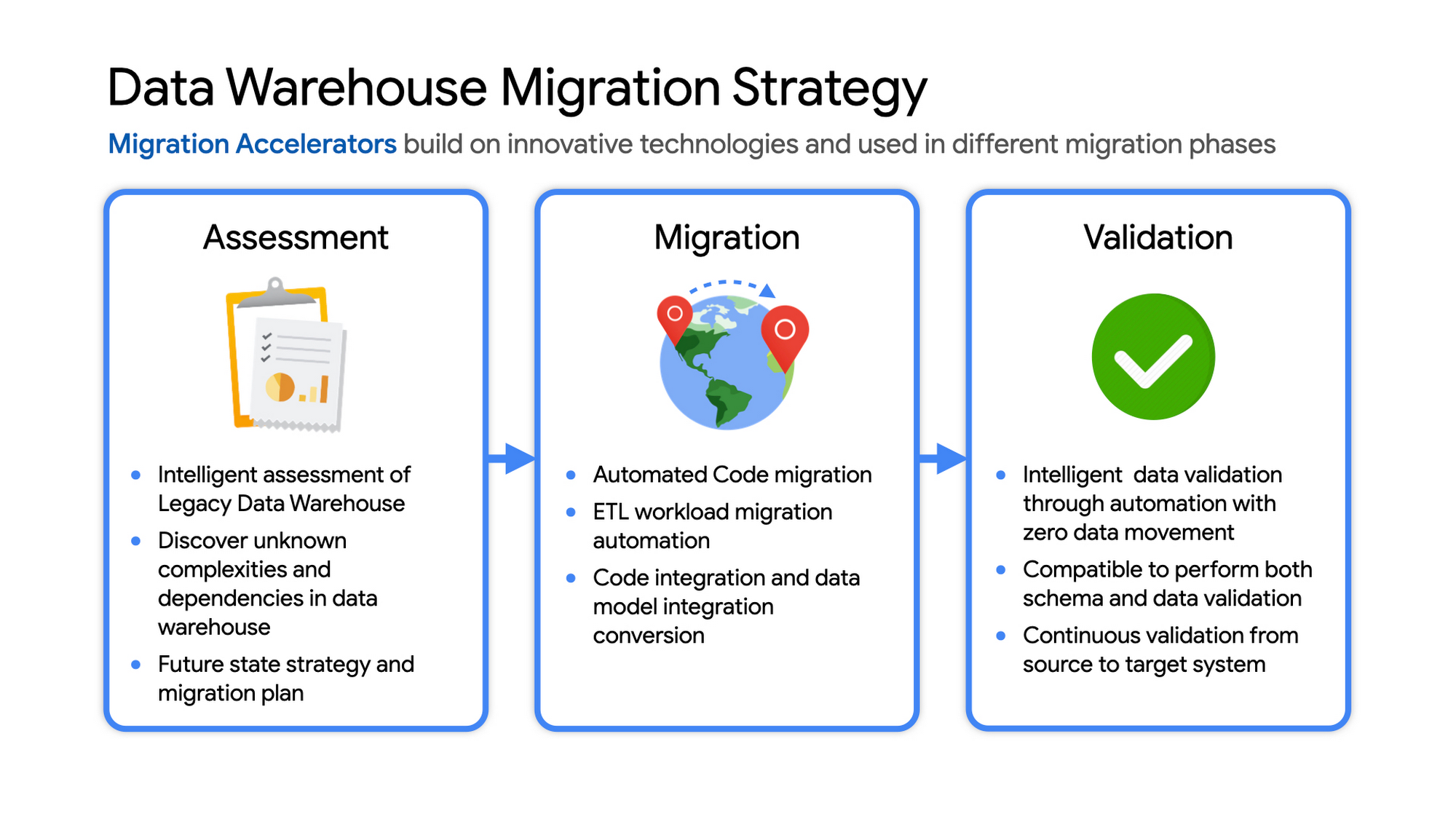
Data warehouse migration strategy
The following steps are typical for a successful migration:
- Assessment and planning: Find the scope in advance to plan the migration of the legacy data warehouse
- Identify data groupings, application access patterns and capacities
- Use tools and utilities to identify unknown complexities and dependencies
- Identify required application conversions and testing
- Determine initial processing and storage capacity for budget forecasting and capacity planning
- Consider growth and changes anticipated during the migration period
- Develop a future state strategy and vision to guide design
- Migration: Establish GCP foundation and begin migration
- As the cloud foundation is being set up, consider running focused POCs to validate data migration processes and timelines
- Look for automated utilities to help with any required code migration
- Plan to maintain data synchronization between legacy and target EDW during the duration of the migration. This becomes a critical business process to keep the project on schedule.
- Plan to integrate some enterprise tooling to help existing teams span both environments
- Consider current data access patterns among EDW user communities and how they will map to similar controls available in Big Query.
- Key scope includes code integration and data model conversions
- Expect to refine capacity forecasts and refine allocation design. In Big Query there are many options to balance cost and performance to maximize business value. For example, you can use either on-demand or flat-rate slot pricing or a combination of both.
- Validation and testing
- Look for tools to allow automated, intelligent data validation
- Scope must include both schema and data validation
- Ideally solutions will allow continuous validation from source to target system during migration
- Testing complexity and duration will be driven by number and complexity of applications consuming data from the EDW and rate of change of those applications
A key to successful migration is finding Google Cloud partners with experience migrating EDW workloads. For example, our Google Cloud partner Datametica offers services and specialized Migration Accelerators for each of these migration stages to make it more efficient to plan and execute migrations.
Data warehouse migration: Things to consider
- Financial benefits of open source: Target moving to ‘Open Source’ where none of the services have license fees. For example BigQuery uses Standard SQL; Cloud Composer is managed Apache Airflow, Dataflow is based on Apache Beam. Taking these as managed services provides the financial benefits of open source, but avoids the burden of maintaining open source platforms internally.
- Serverless: Move to “serverless” big data services. The majority of the services used in a recommended GCP data architecture scale on demand allowing more cost effective alignment with needs. Using fully managed services lets you focus engineering time on business roadmap priorities, not building and maintaining infrastructure.
- Efficiencies of a Unified platform: Any data warehouse migration involves integration with services that surround the EDW for data ingest and pre-processing and advanced analytics on the data stored in the EDW to maximize business value. A cloud provider like GCP offers a full breadth of integrated and managed ‘big data’ services with built-in machine learning. This can yield significantly reduced long-term TCO by increasing both operational and cost efficiency when compared to EDW-specific point solutions.
- Establishing a solid cloud foundation: From the beginning, take the time to design a secure foundation that will serve the business and technical needs for workloads to follow. Key features include: Scalable Resource Hierarchy, Multi-layer security, multi-tiered network and data center strategy and automation using Infrastructure-as-Code. Also allow time to integrate cloud-based services into existing enterprise systems such as CI/CD pipelines, monitoring, alerting, logging, process scheduling, and service request management.
- Unlimited expansion capacity: Moving to cloud sounds like a major step, but really look at this as adding more data centers accessible to your teams. Of course, these data centers offer many new services that are very difficult to develop in-house and provide nearly unlimited expansion capacity with minimal up-front financial commitment. .
- Patience and interim platforms: Migrating an EDW is typically a long running project. Be ready to design and operate interim platforms for data synchronization, validation and application testing. Consider the impact on up-stream and down-stream systems. It might make sense to migrate and modernize these systems concurrent with the EDW migration since they are probably data sources and sinks and may be facing similar growth challenges. Also be ready to accommodate new business requirements that develop during the migration. Take advantage of the long duration to have existing your operational teams learn new services from the partner leading the deployment so your teams are ready to take over post-migration.
- Experienced partner: An EDW migration can be a major undertaking with challenges and risks during migration, but offers tremendous opportunities to reduce costs, simplify operations and offer dramatically improved capacities to internal and external EDW users. Selecting the right partner reduces the technical and financial risks, and allows you to plan for and possibly start leveraging these long-term benefits early in the migration process.
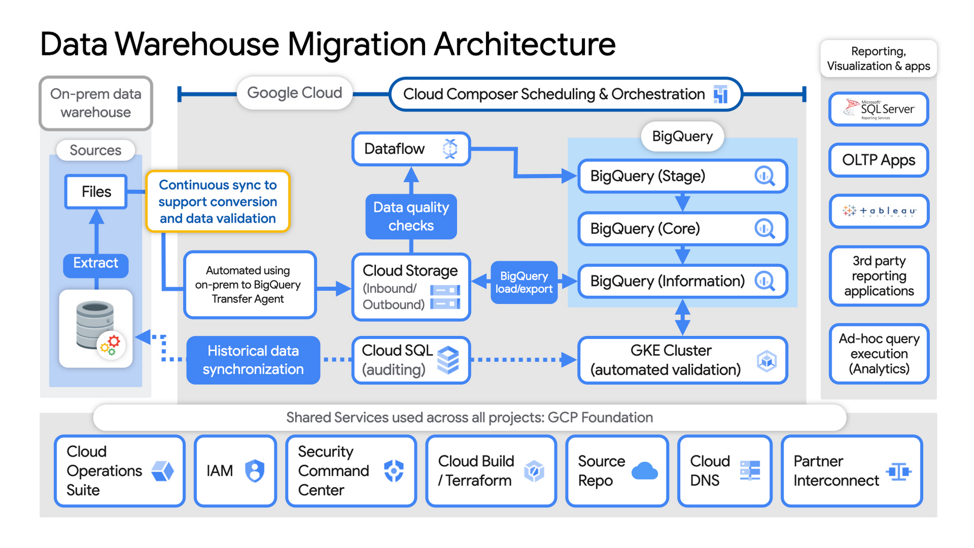
Example Data Warehouse Migration Architecture
- Setup foundational elements. In GCP these include, IAM for authorization and access, cloud resource hierarchy, billing, networking, code pipelines, Infrastructure as Code using Cloud Build with Terraform ( GCP Foundation Toolkit), Cloud DNS and a dedicated/partner Interconnect to connect to the current data centers.
- Activate monitoring and security scanning services before real user data is loaded using Cloud Operations for monitoring and logging and Security Command Center for security monitoring.
- Extract files from on-premise legacy EDW and move to Cloud Storage and establish on-going synchronization using Big Query Transfer services.
- From Cloud Storage, process the data in Dataflow and Load/Export data to BigQuery.
- Validate the export using Datametica’s validation utilities running in a GKE cluster and Cloud SQL for auditing and historical data synchronization as needed. Application teams test against the validated data sets throughout the migration process.
- Orchestrate the entire pipeline using Cloud Composer, integrated with on-prem scheduling services as needed to leverage established processes and keep legacy and new systems in sync.
- Maintain close coordination with teams/services ingesting new data into the EDW and down-streams analytics teams relying on the EDW data for on-going advanced analytics.
- Establish fine-grained access controls to data sets and start making the data in Big Query available to existing reporting, visualization and application consumption tools using BigQuery data connectors for ‘down-stream’ user access and testing.
- Incrementally increase Big Query flat-rate processing capacity to provide the most cost-effective utilization of resources during migration.
To learn more about migrating from on-premises Enterprise Data Warehouses (EDW) to Bigquery and GCP here.
More Relevant Stories for Your Company

How Arvind Fashions Ltd leads the fashion industry with powerful data analytics on BigQuery
Arvind Ltd has been in the apparel industry for more than 90 years, with its retail powerhouse Arvind Fashions Ltd being the backbone of well-known names in the retail fashion industry in India. Arvind Fashions Ltd (Arvind) has seen significant growth in its portfolio with new franchises being added every

Fortress Vault Joins Forces with Google Cloud: Launches Private Data Storage for NFTs
Over the past two years, the general population has become more acquainted with cryptocurrencies and the first iterations of NFTs, which were among the earliest use cases for blockchain technology. This public awareness and participation has led to a growing interest in, and demand for, Web3 technology at the enterprise

What is BigQuery?
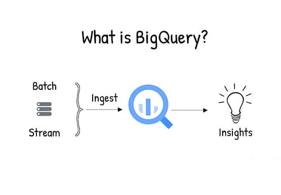
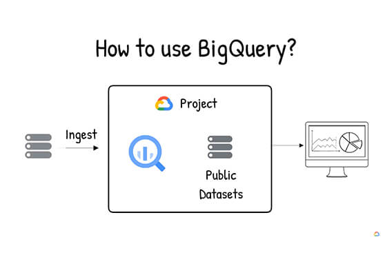
BigQuery is Google Cloud's enterprise data warehouse designed to help you ingest, store, analyze, and visualize big data with ease. Organizations rely on data warehouses to aggregate data from disparate sources, process it, and make it readily available for data analysis that supports their strategic decision-making. You can ingest data

Google Data Cloud: The Catalyst for Modern App Development and Innovation
97 zettabytes was the estimated volume of data generated worldwide in 20221. This sort of explosion in data volume is happening in every enterprise. Now imagine being able to access all this data you own from anywhere, at any time, analyze it, and leverage its insights to innovate your products
