





Experts’ Guideline for Personalizing Platforms with the Right Recommendation System on Google Cloud

5016
Of your peers have already read this article.
5:00 Minutes
The most insightful time you'll spend today!
Over the past two decades, consumers have become accustomed to receiving personalized recommendations in all facets of their online life. Whether that be recommended products while shopping on Amazon, a curated list of apps in the Google Play store, or relevant videos to watch next on YouTube. In fact, in a Verge article “How YouTube perfected the feed: Google Brain gave YouTube new life,” the Google Brain team reveals how their recommendation engine has impacted the platform with “more than 70 percent of the time people spend watching videos on the site being driven by YouTube’s algorithmic recommendations” thereby increasing time spent on the platform by 20X in three years.
It’s become clear that personalized recommendations are no longer a differentiator for an organization but rather something consumers have come to expect in their day-to-day experiences online. So what should you do if you are behind the curve and want to get started or simply want to improve upon what you already have? While there are all sorts of techniques, from content-based systems to deep learning methods, our goal in this recommender-focused blog series is to demystify three available approaches to building recommendation systems on Google Cloud: Matrix Factorization in BigQuery Machine Learning (BQML), Recommendations AI, and deep retrieval techniques available via the Two-Tower built-in algorithm.
One of these approaches can be used to meet you where you are in your personalization journey, no matter if you are just starting or if you are well into it. This first blog post will introduce our three approaches and when to use them.
What is Matrix Factorization and how does it work?
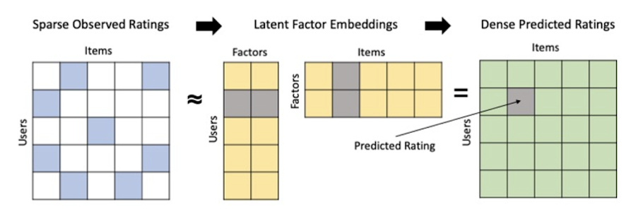
Collaborative filtering is a foundational model for building a recommendation system as the input dataset is simple and the embeddings are learned for you. How does Matrix factorization fit into the mix you might be wondering? Matrix factorization is simply the model that applies collaborative filtering. BQML enables users to create and execute a matrix factorization model by using standard SQL directly in the data warehouse.
Collaborative filtering begins by creating an interaction matrix. The interaction matrix represents users as a row and items as columns in your dataset. This interaction matrix often is sparse in nature as not all users will have interacted with many items in your catalog. This is where embeddings come into play. Generating embeddings for users and items not only allows you to collapse many sparse features into a lower dimensional space but they also allow you to derive a similarity measure so that similar users/items fall nearby in the embedding space. These similarity measures are key as collaborative filtering uses similarities between users and items to make the end recommendations. The underlying assumption being that similar users will like similar items whether that be movies or handbags.
What’s required to get started?
To train a matrix factorization model you need a table that includes three input columns: user(s), item(s), and an implicit or explicit feedback variable (e.g., ratings is an example of explicit feedback). With the base input dataset in place, you can then easily run your model in BigQuery after specifying several hyperparameters in your CREATE MODEL SQL statement. Hyperparameters are available to specify the number of embeddings, the feedback type, the amount of L2 regularization applied and so on.
Why use this approach and who is it a good fit for?
As mentioned earlier, Matrix Factorization in BQML is a great way for those new to recommendation systems to get started. Matrix factorization has many benefits:
- Little ML Expertise: Leveraging SQL to build the model lowers the level of ML expertise needed
- Few Input Features: Data inputs are straightforward, requiring a simple interaction matrix
- Additional Insight: Collaborative filtering is adept at discovering new interests or products for users
While Matrix Factorization is a great tool for deriving recommendations it does come with additional considerations and potential drawbacks depending upon the use case.
- Not Amenable to Large Feature Sets: The input table can only contain two feature columns (e.g., user(s), item(s)). If there is a need to include additional features such as contextual signals, Matrix factorization may not be the right method for you.
- New Items: If an item is not available in the training data, the system can’t create an embedding for it and will have difficulty recommending similar items. While there are some workarounds available to address this cold-start issue, if your item catalog often includes new items, Matrix factorization may not be a good fit.
- Input Data Limitations: While the input matrix is expected to be sparse, training examples without feedback can cause problems. Filtering for items and users that have at least a handful of feedback (e.g., ratings) examples can improve the model. More information on limitations can be found here.
In summary, for users with a simplified dataset looking to iterate quickly and develop a baseline recommendation system, Matrix Factorization is a great approach to begin your personalization AI journey.
What is Recommendations AI and how does it work?
Recommendations AI is a fully managed service which helps organizations deploy scalable recommendation systems that use state-of-the-art deep learning techniques, including cutting-edge architectures such as two-tower encoders, to serve personalized and contextually relevant recommendations throughout the customer journey.
Deep learning models are able to improve the context and relevance of recommendations in part because they can easily address the previously mentioned limitations of Matrix Factorization. They incorporate a wide set of user and item features, and by definition they emphasize learning successive layers of increasingly meaningful representations from these features. This flexibility and expressivity allows them to capture complex relationships like short-lived fashion trends and niche user behaviors. However, this increased relevance comes at a cost, as deep learning recommenders can be difficult to train and expensive to serve at scale.
Recommendations AI helps organizations take advantage of serving these deep learning models and handles the MLOps required to serve these models globally with low latency. Models are automatically retrained daily and tuned quarterly to capture changes in customer behavior, product assortment, pricing, and promotions. Newly trained models follow a resilient CI/CD routine which validates they are fit to serve and promotes them to production without service interruption. The models achieve low serving latency by using a scalable approximate nearest neighbors (ANN) service for efficient item retrieval at inference time. And, to maintain consistency between online and offline tasks, a scalable feature store is used, preventing common production challenges such as data leakage and training-serving skew.
What’s required to get started?
To get started with Recommendations AI we first need to ingest product and user data into the API:
- Import product catalog: For large product catalog updates, ingest catalog items in bulk using the catalogItems.import method. Frequent catalog updates can be schedule with Google Merchant Center or BigQuery
- Record user events: User events track actions such as clicking on a product, adding items to cart, or even purchasing an item. These events need to be ingested in real time to reflect the latest user behavior and then joined to items imported in the product catalog
- Import historical user events: The models need sufficient training data before they can provide accurate predictions. The recommended user event data requirements are different across model types (learn more here)
Once the data requirements are met, we are able to create one or multiple models to serve recommendations:
- Determine your recommendation types and placements: The location of the recommendation panel and the objective for that panel impact model training and tuning. Review the available recommendations types, optimization objectives, and other model tuning options to determine the best options for your business objectives.
- Create model(s): Initial model training and tuning can take 2-5 days depending on the number of user events and size of the product catalog
- Create serving configurations and preview recommendations: After the model is activated, create serving configurations and preview the recommendations to ensure your setup is functioning as expected before serving to production traffic
Once models are ready to serve, consider setting up A/B experiments to understand how newly trained models impact your customer experience before serving them to 100% of your traffic. In the Recommendations AI console, see the Monitoring & Analytics page for summary and placement-specific metrics (e.g., recommender-engaged revenue, click-through-rate, conversion rate, and more).
Why use this approach and who is it a good fit for?
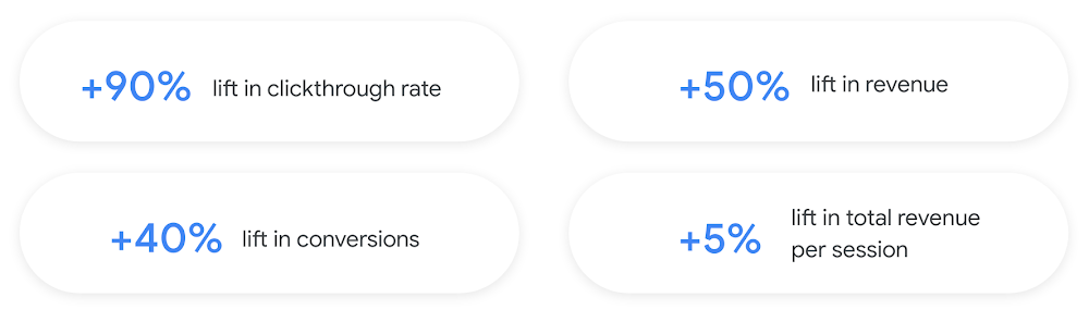
Recommendations AI is a great way to engage customers and grow your online presence through personalization. It’s used by teams who lack technical experience with production recommendation systems, as well as customers who have this technical depth but want to allocate their team’s effort towards other priorities and challenges. No matter your team’s technical experience or bandwidth, you can expect several benefits with Recommendations AI:
- Fully managed service: no need to preprocess data, train or hypertune machine learning models, load balance or manually provision you infrastructure – this is all taken care of for you. The recommendation API also provides a user-friendly console to monitor performance over time.
- State-of-the-art AI: take advantage of the same modeling techniques used to serve recommendations across Google Ads, Google Search, and YouTube. These models excel in scenarios with long-tail products and cold-starts users and items
- Deliver at any touchpoint: serve high-quality recommendations to both first-time users and loyal customers anywhere in their journey via web, mobile, email, and more
- Deliver globally: serve recommendations in any language anywhere in the world at low-latency with a fully automated global serving infrastructure
- Your data, your models: Your data and models are yours. They’ll never be used for any other Google product nor shown to any other Google customer
For users looking to leverage state of the art AI to fuel their recommendation systems but need an existing solution to get up and running more quickly, Recommendations AI is the right solution for you.
What are Two Tower encoders and how do they work?
As a reminder, in recommendation system design, our objective is to surface the most relevant set of items for a given user or set of users. The items are usually referred to as the candidate(s) where we might include information about the items such as the title or description of the item, other metadata about the item like language, number of views, or even clicks on the item over time. User(s) are often represented in the form of a query to a recommendation system where we might provide details about the user such as the location of the user, preferred languages, and what they have searched for in the past.
Let’s start with a common example. Imagine that you are creating a movie recommendation system. The input candidates for such a system would be thousands of movies and the query set can consist of millions of viewers. The goal of the retrieval stage is to select a smaller subset of movies(candidates) for each user and then score and rank order them before presenting the final recommended list to the query/user.
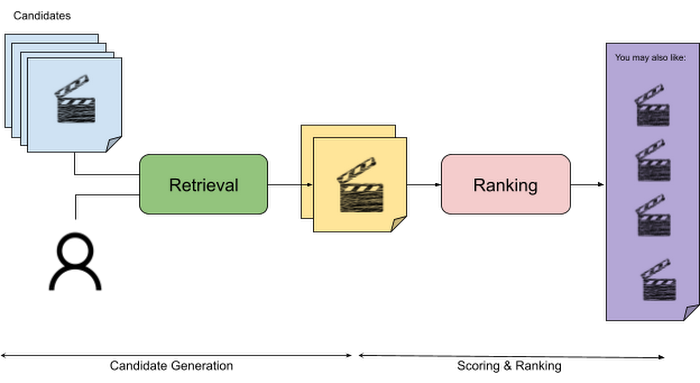
The retrieval stage is able to refine our list of candidates by encoding both the candidate and the query data so they share the same embedding space. A good embedding space will place candidates which are similar to one another closer together and dissimilar items/queries farther apart in the embedding space.
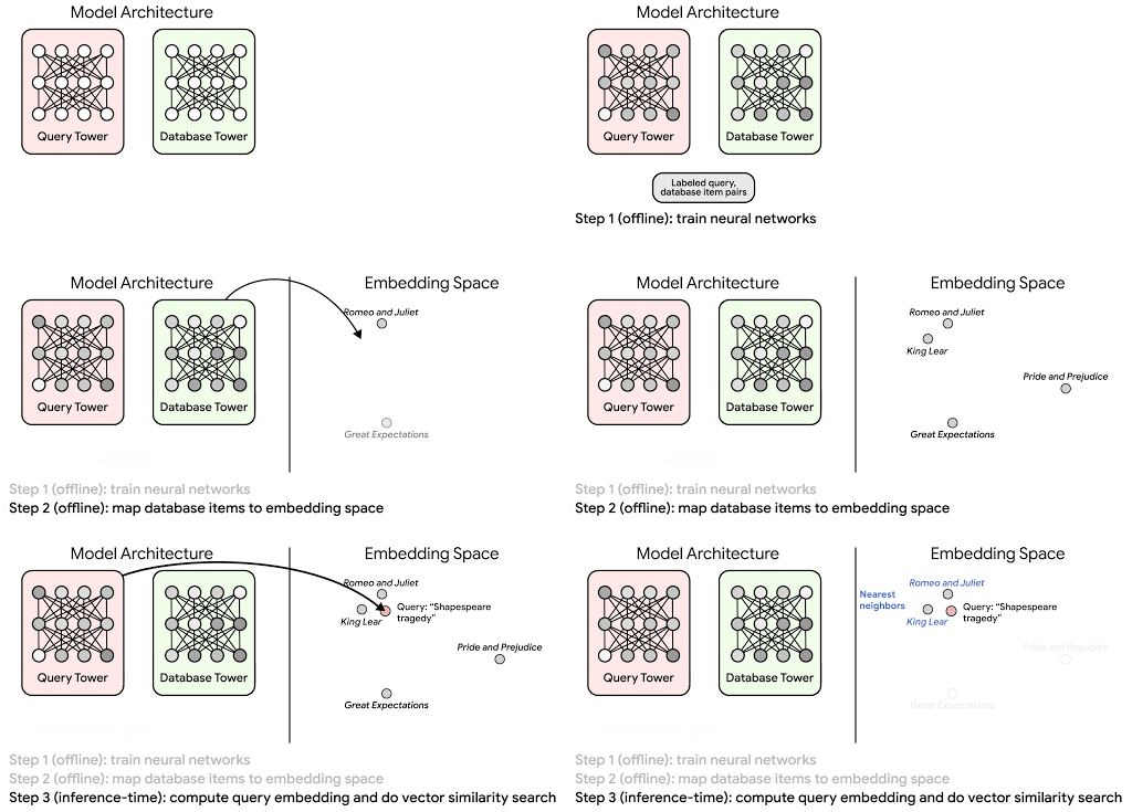
Once we have a database of query and candidate embeddings we can then use an approximate nearest neighbor search method to then generate a list of final “like” candidates, i.e. find a certain number of nearest neighbors for a given query/user and surface final recommendations.
What’s required to get started?
At the most basic level, in order to train a two-tower model you need the following inputs:
- Training Data: Training data is created by combining your query/user data with data about the candidates/items. The data must include matched pairs, cases where both user and item information is available. Data in the training set can include many formats from text, numeric data, or even images.
- Input Schema: The input schema describes the schema of the combined training data along with any specific feature configurations.
Several services within Vertex AI have come available that complement the existing Two-Tower built-in algorithm and can be leveraged in your execution:
- Nearest Neighbor (ANN) Service: Vertex AI Matching Engine and ScANN provide a high-scale and low-latency Approximate Nearest Neighbor (ANN) service so you can more easily identify similar embeddings.
- Hyperparameter Tuning Service: A hyperparameter tuning service such as Vizier can help you identify the optimal hyperparameters such as the number of hidden layers, the size of the hidden layers, and the learning rate in fewer trials.
- Hardware Accelerators: Specialized hardware, such as GPUs or TPUs, can be valuable in your recommendation system to help accelerate experiments and improve the speed of training cycles.
Why use this approach and who is it a good fit for?
The Two-Tower built-in algorithm can be considered the “custom sports car” of recommendation systems and comes with several benefits:
- Greater Control: While Recommendations AI uses the two-tower architecture as one of the available architectures it doesn’t provide granular control or visibility into model training, example generation, and model validation details. In comparison, the Two-Tower built in algorithm provides a more customizable approach as you are training a model directly in a notebook environment.
- More Feature Options: The Two Tower approach can handle additional contextual signals ranging from text to images.
- Cold Start Cases: Leveraging a rich set of features not only enhances performance but also allows the candidate generation to work for new users or new candidates.
While the Two-Tower built in algorithm is an excellent and best-in class solution for deriving recommendations, it does come with additional considerations and potential drawbacks depending upon the use case.
- Technical ML Expertise Required: Two tower encoders are not a “plug and play” solution like the other approaches mentioned above. In order to effectively leverage this approach, appropriate coding and ML expertise is required.
- Speed to Insight: Building out a custom solution via two-tower encoders may require additional time as the solution is not pre-built for the user.
For users looking for greater control, increased flexibility, and have the technical chops to easily work within a managed notebook environment – the two-tower built in algorithm is the right solution for them.
What’s next?
In this article, we explored three common methods for building recommendation systems on Google Cloud Platform. As you can see thus far, there are alot of considerations to take into account before choosing a final approach. In an effort to help you align more quickly we have distilled the decision criteria down to a few simple steps (see below for more details).
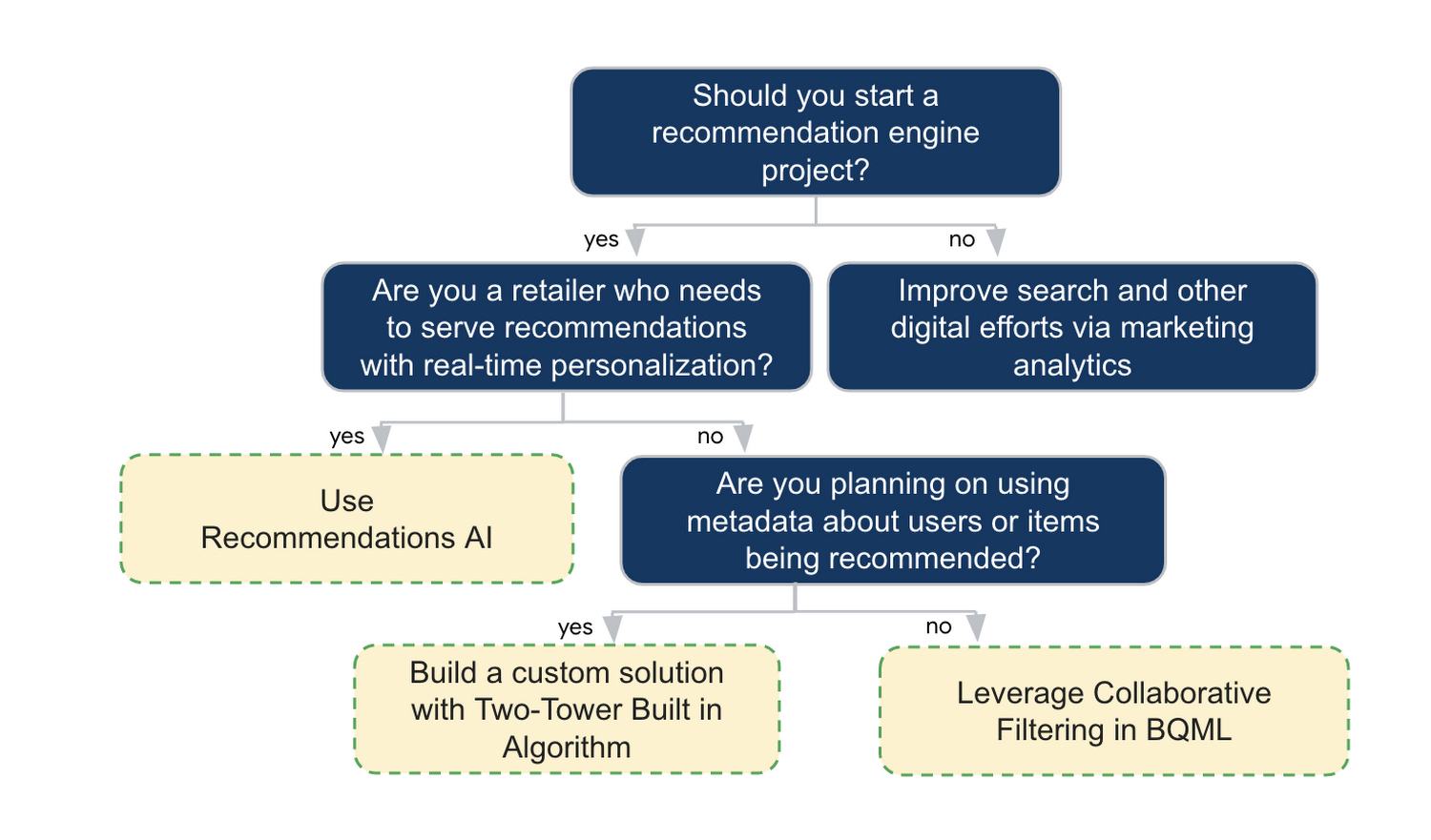
In the next installments of this series, we will dive more deeply into each method, explore how hardware accelerators can play a key role in recommendation system design, and discuss how recommendation systems may be leveraged in key verticals. Stay tuned for future posts in our recommendation systems series. Thank you for reading! Have a question or want to chat? Find authors here – R.E. [Twitter | LinkedIn], Jordan [LinkedIn], and Vaibhav [LinkedIn].
Acknowledgements
Special thanks to Pallav Mehta, Henry Tappen,Abhinav Khushraj, and Nicholas Edelman for helping to review this post.
References
Delivering 10X Improvement to Risk and Regulatory Reporting Through Cloud and AI
5000
Of your peers have already read this article.
2:30 Minutes
The most insightful time you'll spend today!
Enterprise agility and the ability to innovate, adapt and respond quickly to the ever-changing risk and regulatory landscape is no longer a choice, but the cornerstone of successful digital transformation and commercial growth. Traditional access to and ways of managing data invariably create challenges in dealing with multiple data repositories, reconciliations, fire-drills, etc.
In response, the move to cloud is increasing significantly. It enables risk analytics and regulatory reporting at scale in a secure environment with data storage, management and encryption capabilities as a standard. In addition, as regulatory reporting requirements become more granular, machine learning can help facilitate new insights and allow for risk management to become more embedded into operational processes.
This webinar will address the day-to-day challenges in risk management and regulatory compliance, while also exploring how technological innovations can provide massive improvements and potential.
Key themes
- Real-life data challenges in the eyes of risk managers: can compliance, fraud detection and identifying liquidity positions be improved through the use of AI?
- Innovative approaches to streamline regulatory reporting to derive deeper customer insights from data at the moment of truth.
- Reimagining operations: how to modernise the data infrastructure to accommodate data explosion, drive flexibility and deliver a more cost effective outcome.
Make Meaningful Analysis with Geo Boundary Public Datasets on BigQuery

6359
Of your peers have already read this article.
4:00 Minutes
The most insightful time you'll spend today!
Geospatial data is a critical component for a comprehensive analytics strategy. Whether you are trying to visualize data using geospatial parameters or do deeper analysis or modeling on customer distribution or proximity, most organizations have some type of geospatial data they would like to use – whether it be customer zipcodes, store locations, or shipping addresses. However, converting geographic data into the correct format for analysis and aggregation at different levels can be difficult. In this post, we’ll walk through some examples of how you can leverage the Google Cloud platform alongside Google Cloud Public Datasets to perform robust analytics on geographic data. The full queries can be accessed from this notebook here.
Public US Geo Boundaries dataset
BigQuery hosts a slew of public datasets for you to access and integrate into your analytics. Google pays for the storage of these datasets and provides public access to the data via the bigquery-public-data project. You only pay for queries against the data. Plus, the first 1 TB per month is free! These public datasets are valuable on their own, but when joined against your own data they can unlock new analytics use cases and save the team a lot of time.
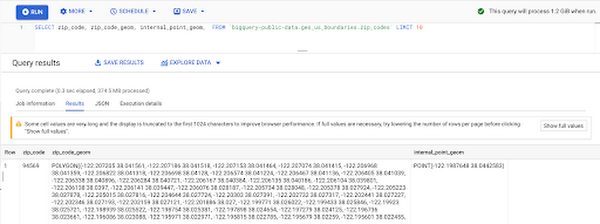
Within the Google Cloud Public Datasets Program there are several geographic datasets. Here, we’ll work with the geo_us_boundaries dataset, which contains a set of tables that have the boundaries of different geospatial areas as polygons and coordinates based on the center point (GEOGRAPHY column type in BigQuery), published by the US Census Bureau.
Mapping geospatial points to hierarchical areas
Many times you will find yourself in situations where you have a string representing an address. However, most tools require lat/long coordinates to actually plot points. Using the Google Maps Geocoding API we can convert an address into a lat/long and then store the results in the BigQuery table.
With a lat/long representation of our point, we can join our initial dataset back onto any of the tables here using the ST_WITHIN function. This allows us to check and see if a point is within the specified polygon.
ST_WITHIN(geography_1, geography_2)
This can be helpful for ensuring standard nomenclature; for example, metropolitan areas that might be named differently. The query below maps each customers’ address to a given metropolitan area name.
SELECTcust.id as customer_id,metro.name as metro_nameFROM `looker-private-demo.retail.customers` as cust,`bigquery-public-data.geo_us_boundaries.metropolitan_divisions` as metroWHERE ST_WITHIN(ST_GEOGPOINT(cust.longitude, cust.latitude),metro.metdiv_geom)
It can also be useful for converting to designated market area (DMA), which is often used in creating targeted digital marketing campaigns.
SELECTcust.id as customer_id,dma.dma_nameFROM `looker-private-demo.retail.customers` as cust,`bigquery-public-data.geo_us_boundaries.designated_market_area` as dmaWHERE ST_WITHIN(ST_GEOGPOINT(cust.longitude, cust.latitude),dma.dma_geom)
Or for filling in missing information; for example, some addresses may be missing zip code which results in incorrect calculations when aggregating up to the zipcode level. By joining onto the zip_codes table we can ensure all coordinates are mapped appropriately and aggregate up from there.
SELECTzip.zip_code,count(distinct cust.id) as unique_customersFROM `looker-private-demo.retail.customers` as cust,`bigquery-public-data.geo_us_boundaries.zip_codes` as zipWHERE ST_WITHIN(ST_GEOGPOINT(cust.longitude, cust.latitude),zip.zip_code_geom)GROUP BY 1
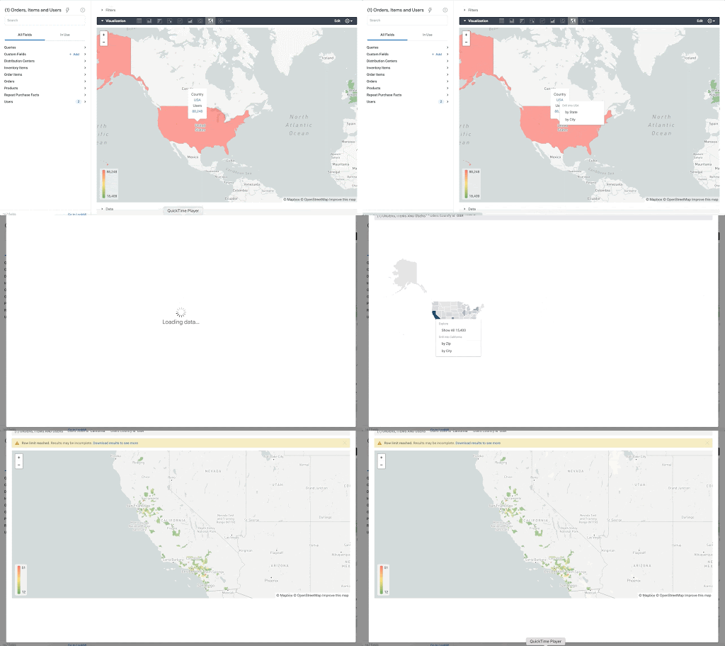
Note that the zip code table isn’t a comprehensive list of all US zip codes, they are zip code tabulation areas (ZCTAs). Details about the differences can be found here. Additionally, the zip code table gives us hierarchical information, which allows us to perform more meaningful analytics. One example is leveraging hierarchical drilling in Looker. I can aggregate my total sales up to the country level, and then drill down to state, city and zipcode to identify where sales are highest. You can also use the BigQuery GeoViz tool to visualize geospatial data!
Aside from simply checking if a point is within an area, we can also use ST_DISTANCE to do something like find the closest city using the centerpoint for the metropolitan area table.
SELECTcust.id as customer_id,ARRAY_AGG(metro.name order by ST_DISTANCE(ST_GEOGPOINT(cust.longitude, cust.latitude),metro.internal_point_geom) asc limit 1)[offset(0)] as metro_nameFROM`looker-private-demo.retail.customers` as cust,`bigquery-public-data.geo_us_boundaries.metropolitan_divisions` as metroGROUP BY cust.id
This concept doesn’t just hold true for points, we can also leverage other GIS functions to see if a geospatial area is contained within areas that are listed in the boundaries datasets. If your data comes into BigQuery as a GeoJSON string, we can convert it to a GEOGRAPHY type using the ST_GEOGFROMGEOJSON function. Once our data is in a GEOGRAPHY type we can do things like check to see what urban area the geo is within – using either ST_WITHIN or ST_INTERSECTS to account for partial coverage. Here, I am using the customer’s zip code to find all metropolitan divisions where the zip code polygon and the metropolitan polygon intersect. I am then selecting the metropolitan area that has the most overlap (or the intersection has the largest area) to be the customer’s metro that we use for reporting.
SELECTcust.id as customer_id,ARRAY_AGG(metro.name order by ST_AREA(ST_INTERSECTION(zip.zip_code_geom,metro.metdiv_geom)) desc limit 1)[offset(0)] as metro_nameFROM`looker-private-demo.retail.customers` as custJOIN `bigquery-public-data.geo_us_boundaries.zip_codes` as zip on cust.zip=zip.zip_code,`bigquery-public-data.geo_us_boundaries.metropolitan_divisions` as metroWHERE ST_INTERSECTS(zip.zip_code_geom,metro.metdiv_geom)GROUP BY cust.id
The same ideas can be applied to the other tables in the dataset including the county, urban areas and National Weather Service forecast regions (which can also be useful if you want to join your datasets onto weather data).
Correcting for data discrepancy
One problem that we may run into when working with geospatial data is that different data sources may have different representations of the same information. For example, you might have one system that records state as a two letter abbreviation and another using the full name. Here, we can use the state table to join the different datasets.
SELECTst.state_name,sum(ab.sales+fn.sales) as total_salesFROM `bigquery-public-data.geo_us_boundaries.states` as stLEFT JOIN abbreviated_table as ab on ab.state = st.stateLEFT JOIN fullname_table as fn on fn.state = st.state_nameWHERE COALESCE(ab.state, fn.state) IS NOT NULLGROUP BY 1
Another example might be using the tables as a source of truth for fuzzy matching. If the address is a manually entered field somewhere in your application, there is a good chance that things will be misspelled. Different representations of the same name may prevent tables from joining with each other or lead to duplicate entries when performing aggregations. Here, I use a simple Soundex algorithm to generate a code for each county name, using helper functions from this blog post. We can see that even though some are misspelled they have the same Soundex code.
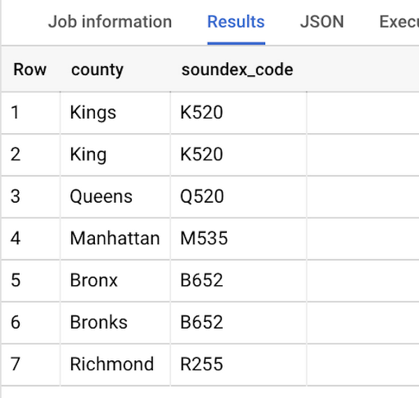
Next, we can join back onto our counties table so we make sure to use the correct spelling of the county name. Then, we can simply aggregate our data for more accurate reporting.
SELECTc.county_name,sum(sales) as total_salesFROMtableJOIN `bigquery-public-data.geo_us_boundaries.counties` as con testing.dq_fm_Soundex(table.county) = testing.dq_fm_Soundex(c.county_name)WHERE c.state_fips_code = cast(36 as string)GROUP BY 1
Note that fuzzy matching definitely isn’t perfect and you might need to try different methods or apply certain filters for it to work best depending on the specifics of your data.
The US Geo Boundary datasets allow you to perform meaningful geographic analysis without needing to worry about extracting, transforming or loading additional datasets into BigQuery. These datasets, along with all the other Google Cloud Public Datasets, will be available in the Analytics Hub. Please sign up for the Analytics Hub preview, which is scheduled to be available in the third quarter of 2021, by going to g.co/cloud/analytics-hub.
3263
Of your peers have already watched this video.
24:00 Minutes
The most insightful time you'll spend today!
An Introduction to MLOps on Google Cloud
The enterprise machine learning life cycle is expanding as firms increasingly look to automate their production ML systems.
MLOps is an ML engineering culture and practice that aims at unifying ML system development and ML system operation enabling shorter development cycles, increased deployment velocity, and more dependable releases in close alignment with business objectives.
In this video, Nate Keating, Product Manager, Google Cloud, will define and give an overview of MLOps and the discuss the challenges at play. He then shares where data science teams are today and where Google Cloud sees them going. Finally he will demonstrate a simple framework for MLOps based on real processes that he has seen in practice.
Learn how to construct your systems to standardize and manage the life cycle of machine learning in production with MLOps on Google Cloud.
How Google Cloud’s Scalable Data Storage and High Compute Resources Fuel Investment Research

6307
Of your peers have already read this article.
1:30 Minutes
The most insightful time you'll spend today!
Investment management is a heavily data-driven industry—portfolio managers and investment researchers require a large number of data sources to guide them in shaping their investment strategies.
New cloud capabilities and technologies enable investment managers to process data faster than ever before and iterate on ideas quickly to fuel innovation in the signal generation process and gain a competitive edge.
Using the cloud for investment research workflows makes it easier to onboard data from data providers, spin up large compute workloads in the midst of market volatility or during heavy research cycles, and manage complex machine learning or natural language workflows to gain market insights.
We hear from industry leaders that they’re exploring new ways to run investment research. “Differentiated investment strategies require new types of information sources, and new ways to process that information,” David Easthope, senior analyst, Market Structure and Technology, Greenwich Associates. “And that, of course, relies heavily on having access to reliable and scalable storage, computational, and AI / ML resources. More specifically, quantitative strategies can benefit from the computational platforms and embedded AI/ML capabilities the cloud can offer.”
Google Cloud gives investment managers essential components to work and operate faster as they bring their investment research workflows to the cloud. Here are the key highlights:
1. Simplify, speed up your data acquisition, discovery, and analytics
The foundation of any investment strategy starts with data—acquiring it, detecting patterns, and analyzing it for insights. Enabling data providers to easily share large datasets such as tick history within a high-performance analytics engine can greatly reduce the data engineering overhead when possible.
Once data is onboarded, you can tag business and technical metadata related to your datasets and provide portfolio managers the ability to discover these datasets via a search interface.
We further review analytics options for various scenarios, including aggregating massive datasets, creating dashboards, and incorporating streaming analytics workloads.
2. Take advantage of burst compute workloads
Data engineers and researchers require ready access to burst compute capabilities to perform backtesting, portfolio simulations and run risk calculations. Cloud works well for these workloads due to its elasticity, consumption-based models, and hardware evolution.
Many investment managers are shifting to a container-based strategy along with a Kubernetes-based scheduler for greater consistency, scaling and efficiency in environments with a large number of researchers. Cloud managed services and a rich suite of CI/CD tools can make this vision a reality while improving security and developer productivity.
3. Tackle machine learning (ML) and model deployment with the help from cloud
Quantitative researchers scour vast amounts of market and alternative data sources searching for signals and correlations, while ML engineers have the challenge of taking these signals and moving them to production.
Google Cloud empowers users to create and operationalize their models without wasting valuable time with a comprehensive set of MLOps tools.
In this paper, we explore multiple solutions for ML and model deployment. Those capabilities reduce the amount of time operationalizing ML models, so quants and data scientists have more time to devote to differentiating activities.
4. Get the data you need in less time with Natural Language and Document AI
Thousands of financial filings, news articles, and sell-side research reports are generated every day, and it’s difficult for humans alone to process this volume of information. These documents are often generated in many languages and the ability to do entity recognition, sentiment or syntactical analysis in those languages, or perhaps translate them into the language of the portfolio manager is of critical importance. Google Cloud provides these capabilities through pre-trained models, or allows you to train high-quality models with your own datasets.
Getting started
There are plenty of emerging technologies, tools, and approaches available to help investment managers today. At Google Cloud, we can help you access, organize, and utilize these essential components to make your research faster, reliable, and more valuable.
To learn more about these four keys to better investment research, check out our whitepaper for more.
Build A Movie Recommender System based on Reinforcement Learning (RL) with Vertex AI

3332
Of your peers have already read this article.
3:00 Minutes
The most insightful time you'll spend today!
Reinforcement learning (RL) is a form of machine learning whereby an agent takes actions in an environment to maximize a given objective (a reward) over this sequence of steps. Applications of RL include learning-based robotics, autonomous vehicles and content serving. The fundamental RL system includes many states, corresponding actions, and rewards to those actions. Translate that into a movie recommender system: The ‘state’ is the user, the ‘action’ is the movie to recommend to the user, and the ‘reward’ is the user rating of the movie. RL is a great framework for optimizing ML models, as mentioned by Spotify in the keynote in the Applied ML Summit 2021.
In this article, we’ll demonstrate an RL-based movie recommender system executed in Vertex AI and built with TF-Agents, a library for RL in TensorFlow. This demo has two parts: (1) a step-by-step guide leveraging Vertex Training, Hyperparameter Tuning, and Prediction services; (2) a MLOps guide to build end-to-end pipelines using Vertex Pipelines and other Vertex services.
TF-Agents meets Vertex AI
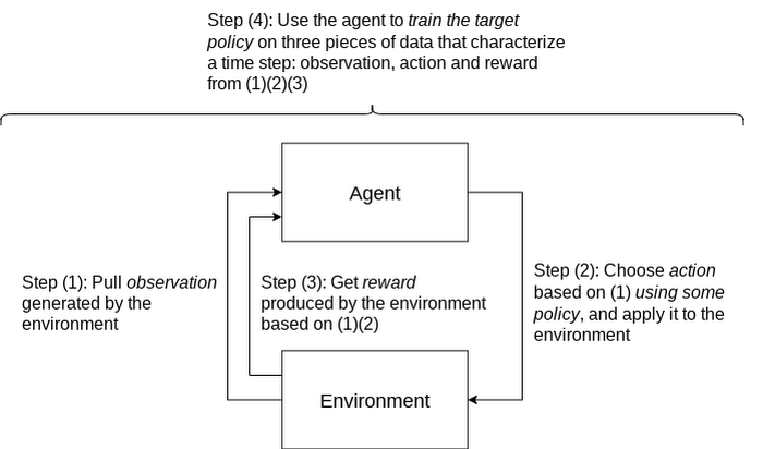
In reinforcement learning (RL), an agent takes a sequence of actions in a given environment according to some policy, with the goal of maximizing a given reward over this sequence of actions. TF-Agents is a powerful and flexible library enabling you to easily design, implement and test RL applications. It provides you with a comprehensive set of logical modules that support easy customization:
- Policy: A mapping from an environment observation to an action or a distribution over actions. It is the artifact produced from training, and the equivalent of a “Model” in a supervised learning setup.
- Action: A move or behavior that is outputted by some policy, and chosen and taken by an agent.
- Agent: An entity that encapsulates an algorithm to use one or more policies to choose and take actions, and trains the policy.
- Observations: A characterization of the environment state.
- Environment: Definition of the RL problem to solve. At each time step, the environment generates an observation, bears the effect of the agent action, and then given the action taken and the observation, the environment responds with a reward as feedback.
A typical RL training loop looks like the following:
A typical process to build, evaluate, and deploy RL applications would be:
- Frame the problem: While this blog post introduces a movie recommendation system, you can use RL to solve a wide range of problems. For instance, you can easily solve a typical classification problem with RL, where you can frame predicted classes as actions. One example would be digit classification: observations are digit images, actions are 0-9 predictions and rewards indicate whether the predictions match the ground truth digits.
- Design and implement RL simulated experiments: We will go into detail on simulated training data and prediction requests in the end-to-end pipeline demo.
- Evaluate performance of the offline experiments.
- Launch end-to-end production pipeline by replacing the simulation constituents with real-world interactions.
Now that you know how we’ll build a movie recommendation system with RL, let’s look at how we can use Vertex AI to run our RL application in the cloud. We’ll use the following Vertex AI products:
- Vertex AI training to train a RL policy (the counterpart of a model in supervised learning) at scale
- Vertex AI hyperparameter tuning to find the best hyperparameters
- Vertex AI prediction to serve trained policies at endpoints
- Vertex Pipelines to automate, monitor, and govern your RL systems by orchestrating your workflow in a serverless manner, and storing your workflow’s artifacts using Vertex ML Metadata.
Step-by-step RL demo
This step-by-step demo showcases how to build the MovieLens recommendation system using TF-Agents and Vertex AI services, primarily custom training and hyperparameter tuning, custom prediction and endpoint deployment. This demo is available on Github, including a step-by-step notebook and Python modules.
The demo first walks through the TF-Agents on-policy (which is covered in detail in the demo) training code of the RL system locally in the notebook environment. It then shows how to integrate the TF-Agents implementation with Vertex AI services: It packages the training (and hyperparameter tuning) logic in a custom training/hyperparameter tuning container and builds the container with Cloud Build. With this container, it executes remote training and hyperparameter tuning jobs using Vertex AI. It also illustrates how to utilize the best hyperparameters learned from the hyperparameter tuning job during training, as an optimization.
The demo also defines the prediction logic, which takes in observations (user vectors) from prediction requests and outputs predicted actions (movie items to recommend), in a custom prediction container and builds the container with Cloud Build. It deploys the trained policy to a Vertex AI endpoint, and uses the prediction container as the serving container for the policy at the Vertex AI endpoint.
End-to-end workflow with a closed feedback loop: Pipeline demo
Pipeline architecture
Building upon our RL demo, we’ll now show you how to scale this workflow using Vertex Pipelines. This pipeline demo showcases how to build an end-to-end MLOps pipeline for the MovieLens recommendation system, using Kubeflow Pipelines (KFP) for authoring and Vertex Pipelines for orchestration.
Highlights of this end-to-end demo include:
- RL-specific implementation that handles RL modules, training logic and trained policies as opposed to models
- Simulated training data, simulated environment for predictions and re-training
- Closing of the feedback loop from prediction results back to training
- Customizable and reproducible KFP components
An illustration of the pipeline structure is shown in the figure below.
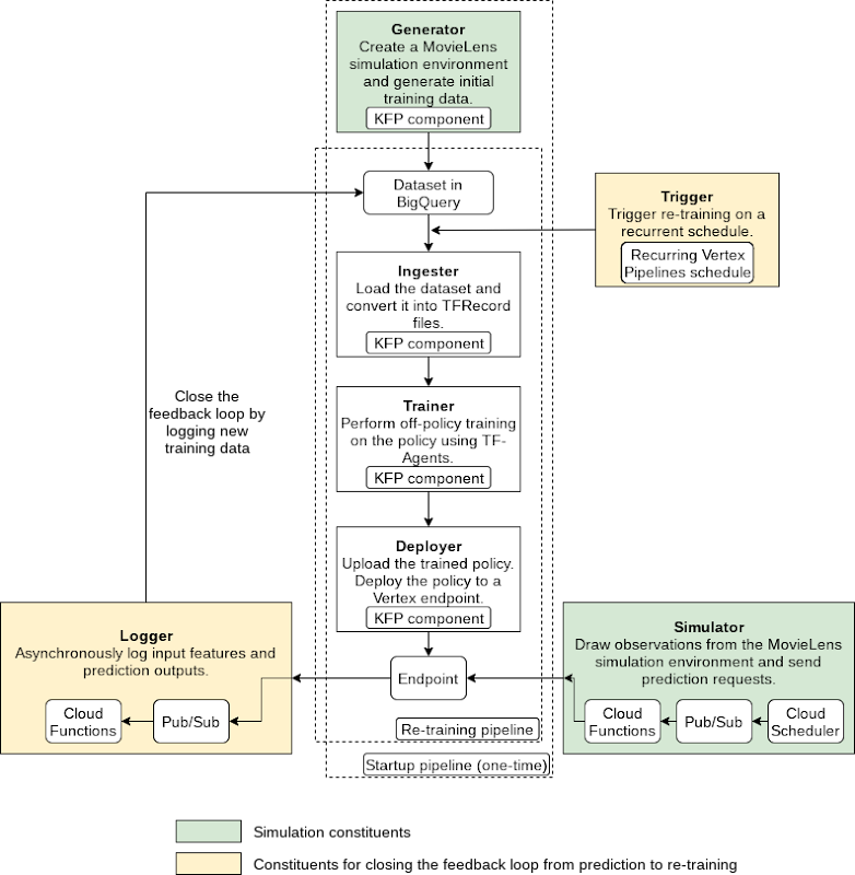
The pipeline consists of the following components:
- Generator: to generate MovieLens simulation data as the initial training dataset using a random data-collecting policy, and store in BigQuery [executed only once]
- Ingester: to ingest training data in BigQuery and output TFRecord files
- Trainer: to perform off-policy (which is covered in detail in the demo) training using the training dataset and output a trained RL policy
- Deployer: to upload the trained policy, create a Vertex AI endpoint and deploy the trained policy to the endpoint
In addition to the above pipeline, there are three components which utilize other GCP services (Cloud Functions, Cloud Scheduler, Pub/Sub):
- Simulator: to send recurring simulated MovieLens prediction requests to the endpoint
- Logger: to asynchronously log prediction inputs and results as new training data back to BigQuery, per prediction requests
- Trigger: to recurrently execute re-training on new training data
Pipeline construction with Kubeflow Pipelines (KFP)
You can author the pipeline using the individual components mentioned above:
@dsl.pipeline(pipeline_root=PIPELINE_ROOT,name=f"{PIPELINE_NAME}-startup")def pipeline(# Pipeline configsproject_id: str,raw_data_path: str,training_artifacts_dir: str,# BigQuery configsbigquery_dataset_id: str,bigquery_location: str,bigquery_table_id: str,bigquery_max_rows: int = 10000,# TF-Agents RL configsbatch_size: int = 8,rank_k: int = 20,num_actions: int = 20,driver_steps: int = 3,num_epochs: int = 5,tikhonov_weight: float = 0.01,agent_alpha: float = 10) -> None:"""Authors a RL pipeline for MovieLens movie recommendation system.Integrates the Generator, Ingester, Trainer and Deployer components. Thispipeline generates initial training data with a random policy and runs onceas the initiation of the system.Args:project_id: GCP project ID. This is required because otherwise the BigQueryclient will use the ID of the tenant GCP project created as a result ofKFP, which doesn't have proper access to BigQuery.raw_data_path: Path to MovieLens 100K's "u.data" file.training_artifacts_dir: Path to store the Trainer artifacts (trained policy).bigquery_dataset: A string of the BigQuery dataset ID in the format of"project.dataset".bigquery_location: A string of the BigQuery dataset location.bigquery_table_id: A string of the BigQuery table ID in the format of"project.dataset.table".bigquery_max_rows: Optional; maximum number of rows to ingest.batch_size: Optional; batch size of environment generated quantities eg.rewards.rank_k: Optional; rank for matrix factorization in the MovieLens environment;also the observation dimension.num_actions: Optional; number of actions (movie items) to choose from.driver_steps: Optional; number of steps to run per batch.num_epochs: Optional; number of training epochs.tikhonov_weight: Optional; LinUCB Tikhonov regularization weight of theTrainer.agent_alpha: Optional; LinUCB exploration parameter that multiplies theconfidence intervals of the Trainer."""# Run the Generator component.generate_op = create_component_from_func(func=generator_component.generate_movielens_dataset_for_bigquery,output_component_file=f"generator-{OUTPUT_COMPONENT_SPEC}",packages_to_install=["google-cloud-bigquery==2.20.0","tensorflow==2.5.0","tf-agents==0.8.0",])generate_task = generate_op(project_id=project_id,raw_data_path=raw_data_path,batch_size=batch_size,rank_k=rank_k,num_actions=num_actions,driver_steps=driver_steps,bigquery_tmp_file=BIGQUERY_TMP_FILE,bigquery_dataset_id=bigquery_dataset_id,bigquery_location=bigquery_location,bigquery_table_id=bigquery_table_id)# Run the Ingester component.ingest_op = create_component_from_func(func=ingester_component.ingest_bigquery_dataset_into_tfrecord,output_component_file=f"ingester-{OUTPUT_COMPONENT_SPEC}",packages_to_install=["google-cloud-bigquery==2.20.0","tensorflow==2.5.0",])ingest_task = ingest_op(project_id=project_id,bigquery_table_id=generate_task.outputs["bigquery_table_id"],bigquery_max_rows=bigquery_max_rows,tfrecord_file=TFRECORD_FILE)# Run the Trainer component and submit custom job to Vertex AI.train_op = create_component_from_func(func=trainer_component.training_op,output_component_file=f"trainer-{OUTPUT_COMPONENT_SPEC}",packages_to_install=["tensorflow==2.5.0","tf-agents==0.8.0",])train_task = train_op(training_artifacts_dir=training_artifacts_dir,tfrecord_file=ingest_task.outputs["tfrecord_file"],num_epochs=num_epochs,rank_k=rank_k,num_actions=num_actions,tikhonov_weight=tikhonov_weight,agent_alpha=agent_alpha)worker_pool_specs = [{"containerSpec": {"imageUri":train_task.container.image,},"replicaCount": TRAINING_REPLICA_COUNT,"machineSpec": {"machineType": TRAINING_MACHINE_TYPE,"acceleratorType": TRAINING_ACCELERATOR_TYPE,"acceleratorCount": TRAINING_ACCELERATOR_COUNT,},},]train_task.custom_job_spec = {"displayName": train_task.name,"jobSpec": {"workerPoolSpecs": worker_pool_specs,}}# Run the Deployer components.# Upload the trained policy as a model.model_upload_op = gcc_aip.ModelUploadOp(project=project_id,display_name=TRAINED_POLICY_DISPLAY_NAME,artifact_uri=training_artifacts_dir,serving_container_image_uri=f"gcr.io/{PROJECT_ID}/{PREDICTION_CONTAINER}:latest",)# Model uploading has to occur after training completes.model_upload_op.after(train_task)# Create a Vertex AI endpoint. (This operation can occur in parallel with# the Generator, Ingester, Trainer components.)endpoint_create_op = gcc_aip.EndpointCreateOp(project=project_id,display_name=ENDPOINT_DISPLAY_NAME)# Deploy the uploaded, trained policy to the created endpoint. (This operation# has to occur after both model uploading and endpoint creation complete.)model_deploy_op = gcc_aip.ModelDeployOp(project=project_id,endpoint=endpoint_create_op.outputs["endpoint"],model=model_upload_op.outputs["model"],deployed_model_display_name=TRAINED_POLICY_DISPLAY_NAME,machine_type=ENDPOINT_MACHINE_TYPE)
The execution graph of the pipeline looks like the following:
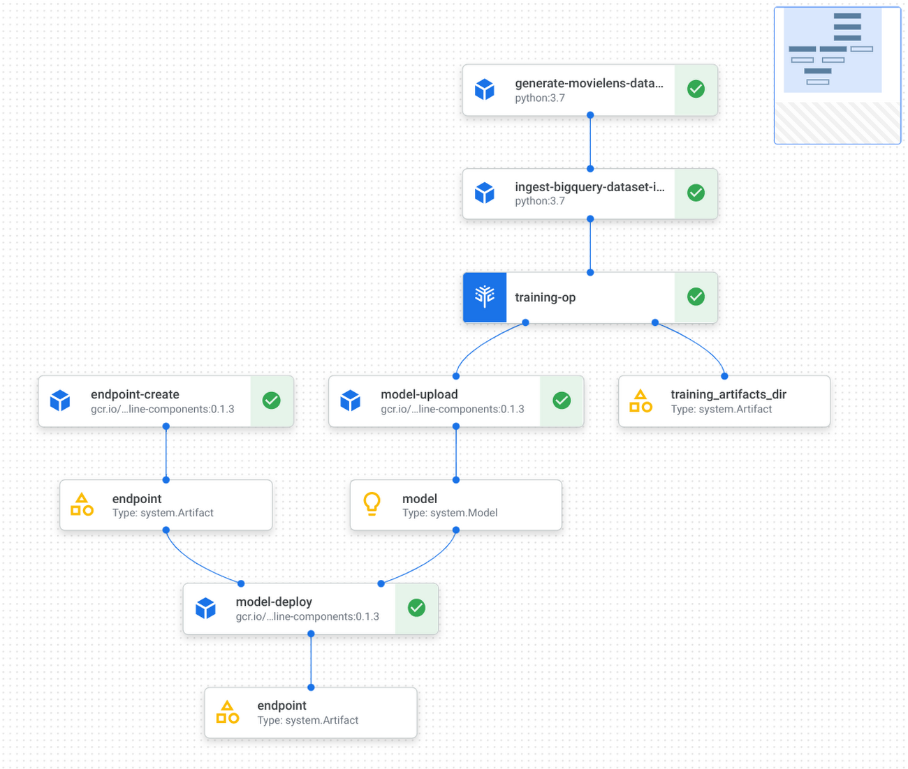
Refer to the GitHub repo for detailed instructions on how to implement and test KFP components, and how to run the pipeline with Vertex Pipelines.
Applying this demo to your own RL projects and production
You can replace the MovieLens simulation environment with a real-world environment where RL quantities like observations, actions and rewards capture relevant aspects of said real-world environment. Based on whether you can interact with the real world in real-time, you may choose either on-policy (showcased by the step-by-step demo) or off-policy (showcased by the pipeline demo) training and evaluation.
If you were to implement a real-world recommendation system, here’s what you’d do:
You would represent users as some user vectors. The individual entries in the user vectors may have actual meanings like age. Alternatively, they may be generated through a neural network as user embeddings. Similarly, you would define what an action is and what actions are possible, likely all items available on your platform; you would also define what the reward is, such as whether the user has tried the item, how long/much the user has spent on the item, user rating of the item, and so on. Again, you have the flexibility to decide on representations for framing the problem that maximize performance. During training or data pre-collection, you may randomly sample users (and build the corresponding user vectors) from the real world, use those vectors as observations to query some policy for items to recommend, and then apply that recommendation to users and obtain their feedback as rewards.
This RL demo can also be extended to ML applications other than recommendation system. For instance, if your use case is to build an image classification system, then you can frame an environment, where observations are the image pixels or embeddings, actions are the predicted classes, and rewards are feedback on the predictions’ correctness.
Conclusion
Congratulations! You have learned how to build reinforcement learning solutions using Vertex AI in a fully managed, modularized and reproducible way. There is so much you can achieve with RL, and you now have many Vertex AI as well as Google Cloud services in your toolbox to support you in your RL endeavors, be it production systems, research or cool personal projects.
Additional resources
- [Recap] step-by-step demo link: GitHub link
- [Recap] end-to-end pipeline demo: GitHub link
- TF-Agents tutorial on bandits: Introduction to Multi-Armed Bandits
- Vertex Pipelines tutorial: Intro to Vertex Pipelines
More Relevant Stories for Your Company

IT Team Figures Out Easiest Way to Build Data Pipelines and Create ML Models
Building a strong brand in today's hyper-competitive business environment takes vision. It also requires a flexible, easily managed approach to digital asset management (DAM), so marketing professionals and other stakeholders can easily share, store, track, and manipulate assets to build the brand. Many of today's leading companies, including JetBlue, Slack,

Discover Gen App Builder: Transform Search and Conversational Experiences Through Generative AI
If you’ve been exploring recently-launched consumer generative AI tools like Bard and thinking about how to build similar experiences for your business, Generative AI App Builder, or Gen App Builder for short, is here to get you started.Gen App Builder is part of Google Cloud’s recently announced generative AI offerings and lets developers,

New Research Shows Top Marketers Use Machine Learning to Drive Growth
Automation and machine learning technologies are changing the way marketers drive results for their customers and brands. But there’s still a significant gap between those who are just talking about machine learning and those who are taking action. For marketers looking to become leaders in their field, this is an

Use No-Cost Solutions To Bring ML Into Your Medical Research
There’s a lot we can learn from combining technology with science to help support the development of amazing discoveries. By using an AI system to predict protein shapes, we have the potential to accelerate research in every field of biology. Inside every cell in your body, billions of tiny molecular
