





BigQuery Now Supports Multi-statement Transactions

3757
Of your peers have already read this article.
3:00 Minutes
The most insightful time you'll spend today!
Mercury, the Roman god of commerce, is often depicted carrying a purse, symbolic of business transactions, wearing winged sandals, illustrating his abilities to move at great speeds. Transactions power the world’s business systems today, ranging from millions of packages moving worldwide tracked in real time by logistics companies to global payments from personal loans to securities trading to intergovernmental transactions, keeping goods and services flowing worldwide. Today, we are very pleased to announce the public preview of multi-statement transactions in BigQuery.
BigQuery has long supported single-statement transactions through DML statements such as INSERT, UPDATE, DELETE, MERGE and TRUNCATE, applied to one table per transaction. Multi-statement transactions expand on this scope by supporting multiple SQL statements, including DML, spanning multiple tables in a single transaction. This means that the changes to data across multiple tables associated with all statements in a given transaction are committed atomically (all at once) if successful or all rolled back atomically in the event of a failure. These new multi-statement transaction capabilities now bridge the gap between online transaction processing (OLTP) systems and BigQuery through tighter and faster integration, just as Mercury’s speed enabled him to travel rapidly between the mortal and divine worlds.
Overview
A transaction is a set of tasks carried out against a database or a data warehouse representing a business unit of work. For example, an order expedite action may result in a series of changes to multiple tables, e.g., updating delivery dates on the order, adding new shipment lines on a shipment to create expedited delivery shipments and canceling (updating) prior normal delivery shipment lines. Correspondingly, when a batch job execute an ETL process in a data warehouse, it may perform data wrangling and data cleansing operations by transforming and saving the data in multiple tables. In both of these cases, if a failure occurs, then the entire transaction must be rolled back so that the system of record does not have partial data saved putting the dataset in an inconsistent state.
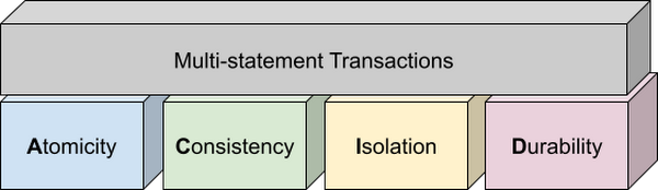
Transactions are known for their atomicity, consistency, isolation, and durability (ACID) properties. Atomicity indicates that all data changes (including metadata changes) are applied or reverted in a single operation, e.g. when a set of rows are added to a table with enrichment and the corresponding set of rows deleted, both operations happen together. Consistency refers to the consistency of data before and after the transaction has completed. When data is added to or updated in a table, the changes to data in tables are consistent with the constraints specified on the table or its columns, e.g. ensuring that the NOT NULL constraint is complied with when data gets added or modified in a table. Isolation indicates that multiple transactions can make changes to the table concurrently as long as the changes don’t conflict with each other, e.g. two transactions loading data into tables from different business units can proceed concurrently. Durability is the last and possibly the most important property of transactions which guarantees that in the event of a failure (after completing the transaction), all the changes committed by the transaction are saved for future transactions or queries.
Isolation level
All transactions in BigQuery including multi-statement transactions support snapshot isolation. At this isolation level, all statements in a transaction see a consistent snapshot of the database, as of the start of the transaction. BigQuery achieves this due to its multi-version property where it maintains the history of mutations to the database for a certain period. Transactions do not see any changes, committed or uncommitted, from other concurrent transactions while the transaction is in progress. BigQuery supports read-your-own-writes, where statements in a transaction can see all the changes applied by prior statements in the same transaction.
Example
Let’s run through an example to demonstrate how BigQuery supports the concept of multi-statement transactions with multiple sets of changes across multiple tables in one operation. In this example, we will set up this demo by creating 10 tables each with 100 partitions
Language: SQL
DECLARE num_tables DEFAULT 10;DECLARE x INT64 DEFAULT 0;# replace "demo" with your preferred dataset nameDECLARE ds STRING default "`00jathreya`";DECLARE prefix STRING DEFAULT "mst_demo";DECLARE table_name STRING;DECLARE pre_table_name STRING;/*Sets up 10 tables, with schema (partition_id:integer,value:timestamp).Each table has 100 partitions, with partition key 0, 10, 20, ..., 990.*/SET x = 0;WHILE x < num_tables DOSET table_name = format("%s.%s_%d", ds, prefix, x);EXECUTE IMMEDIATE format("""DROP TABLE IF EXISTS %s""", table_name);EXECUTE IMMEDIATE format("""CREATE OR REPLACE TABLE %s (partition_id INT64, value TIMESTAMP)PARTITION BY RANGE_BUCKET(partition_id, GENERATE_ARRAY(0, 1000, 10))AS SELECT partition_id, CURRENT_TIMESTAMP() AS value FROM UNNEST(GENERATE_ARRAY(0, 990, 10)) AS partition_id""", table_name);SET x = x + 1;END WHILE;# Verify the partitioned tables created and the timestampexecute immediate format("""select table_schema, table_name, count(partition_id), sum(total_rows), max(last_modified_time) from %s.INFORMATION_SCHEMA.PARTITIONSwhere starts_with(table_name,'%s')group by table_schema, table_name""", ds, prefix);# Verify data in table 9 based on the timestampEXECUTE IMMEDIATE format("""SELECT * FROM %s ORDER BY partition_id""", table_name);
Next, we will show how the new COMMIT and ROLLBACK commands in BigQuery allow you to save or reverse the changes in a transaction spanning multiple tables.
Language: SQL
DECLARE num_tables DEFAULT 10;DECLARE x INT64 DEFAULT 0;# Replace `mydataset` with your preferred dataset nameDECLARE ds STRING DEFAULT "`mydataset`";DECLARE prefix STRING DEFAULT "mst_demo";DECLARE table_name STRING;DECLARE pre_table_name STRING;/*Steps of the transaction:1. For table 0, updates the timestamp to CURRENT_TIMESTAMP.2. FOR table 1 to 9, merge table x using data from table x-1. All MERGE shouldsee the updated data in table x-1, so as a result the change in table 0 should bepropagated all the way to table 9.3. A total of 1000 partition changes on 10 tables.*/BEGIN TRANSACTION;SET x = 0;WHILE x < num_tables DOSET table_name = format("%s.%s_%d", ds, prefix, x);IF x = 0 THENEXECUTE IMMEDIATE format("""UPDATE %s SET value = CURRENT_TIMESTAMP WHERE true""", table_name);ELSESET pre_table_name = format("%s.%s_%d", ds, prefix, x-1);EXECUTE IMMEDIATE format("""MERGE %s t2 USING %s t1 ON t2.partition_id = t1.partition_idWHEN MATCHED THEN UPDATE SET value = t1.value""", table_name, pre_table_name);END IF;SET x = x + 1;END WHILE;# Verify data in table 9 inside transaction shows recently updated dataSET table_name = format("%s.%s_%d", ds, prefix, num_tables-1);EXECUTE IMMEDIATE format("""SELECT * FROM %s ORDER BY partition_id""", table_name);IF x = 9 THENCOMMIT TRANSACTION;ELSEROLLBACK TRANSACTION;END IF;# Verify data in table 9 outside transaction shows timestamp of original dataEXECUTE IMMEDIATE format("""SELECT * FROM %s ORDER BY partition_id""", table_name);
Monitoring and Management
Unlike single-statement transactions which map to a single DML command, multi-statement transactions are complex spanning multiple DML operations across multiple tables. To monitor these complex jobs, the BigQuery JOBS INFORMATION_SCHEMA views have been expanded to add a new column, TRANSACTION_ID, which contains a unique identifier for each transaction in BigQuery. You can query transactions that are in progress or the ones that have completed by querying these views.
Language: SQL
#Returns the list of transactions running under a parent job ID .;SELECTDISTINCT transaction_idFROM `region-us`.INFORMATION_SCHEMA.JOBS_BY_PROJECTWHERE parent_job_id = "job_id" AND state = "RUNNING";# Returns the active transactions and parent job id that are running and affect a named table.;WITHrunning_transactions AS (SELECT DISTINCT transaction_idFROM `region-us`.INFORMATION_SCHEMA.JOBS_BY_PROJECTWHERE state = "RUNNING")SELECTtransaction_id, parent_job_id, queryFROM `region-us`.INFORMATION_SCHEMA.JOBS_BY_PROJECT, running_transactionsWHERE destination_table = "mytable"AND transaction_id = running_transactions.transaction_id;# Returns all successfully committed transactionsSELECTtransaction_id, parent_job_id, queryFROM `region-us`.INFORMATION_SCHEMA.JOBS_BY_PROJECTWHERE statement_type = "COMMIT_TRANSACTION" AND error_result IS NULL;# Returns all rolled back transactionsSELECTtransaction_id, parent_job_id, queryFROM `region-us`.INFORMATION_SCHEMA.JOBS_BY_PROJECTWHERE statement_type = "ROLLBACK_TRANSACTION" AND error_result IS NULL;
To terminate a transaction, you will need to terminate the parent job under which the transaction is running by passing the parent job ID of the script containing the transaction to the BQ.JOBS.CANCEL system procedure.
Conclusion
As enterprises accelerate towards more real time insight-driven decisions, multi-statement transactions are a key enabler towards bringing transaction data into analytical data warehouses, such as BigQuery. With strong ACID properties, full transaction support for commit and rollback, and rich monitoring and management APIs built on proven transaction processing backbone, we are very pleased to help our BigQuery customers unlock the value of transactions through these new capabilities.
Google Cloud Leads the Landscape for Unstructured Data Security Platform: Forrester

7032
Of your peers have already read this article.
1:30 Minutes
The most insightful time you'll spend today!
As organizations expand their use of cloud computing services, more of their sensitive data inevitably moves to and lives in the cloud. Much of this sensitive data is unstructured and can be challenging to secure. Despite this potential challenge, the usefulness of cloud for data storage and processing is too big for most organizations to ignore and has in turn led to data sprawl, where their sensitive data is spread over many resources, both in the cloud and on-premise. Addressing data sprawl requires solutions that can discover, manage, and secure sensitive data, especially unstructured data, as it spreads.
To help organizations confidently move their sensitive data to the cloud, Google Cloud works diligently to earn and maintain customer trust. Control and transparency are pillars of our approach to offering a trusted cloud. Therefore, we’ve been expanding our capabilities to act on unstructured data as sprawl increases.
Given the importance of these capabilities to our strategy, we are happy to announce today that Forrester Research has named Google Cloud a Leader in The Forrester Wave™: Unstructured Data Security Platforms, Q2 2021 report, and rated Google Cloud highest in the current offering category among the providers evaluated.
The report evaluates the 11 most significant providers with platform solutions to secure and protect unstructured data, spanning from cloud providers to data security-focused vendors. The report notes that “Google offers breadth and depth with built-in data security in the cloud. Google Cloud Platform, Google Workspace, and BeyondCorp Enterprise have underlying data security products and features for protecting customer data.”
Google Cloud tools focused on protecting unstructured data were developed and battle-tested internally at Google to alleviate some of our own data security challenges. This brings the best of Google security to the organizations utilizing Google Cloud and our security tools. The report highlights that “Google productizes capabilities originally developed to secure its own business, and brings a disciplined approach to product enhancements for enterprise requirements. It serves a wide range of enterprise and mid-market, with a focus on emphasizing data protection needs by industry. ”
Google Cloud’s data security strategy focuses on meeting customers wherever they are in their cloud migration journey. The report highlights that “Google further enables a Zero Trust approach with third-party integrations through its BeyondCorp Alliance of partners in device management, endpoint security and gateways.”
Google Cloud received the highest possible score in sixteen criteria, in total receiving the most 5 out of 5 ratings among all vendors assessed. These criteria include: Data Intelligence, Access Control, Deletion, Obfuscation-Scope, Obfuscation-Key Management, Deployment, Security and Risk, APIs and Integration, Data Security Platform Vision, Data Security Execution Roadmap, Performance, Planned Enhancements, Zero Trust Enabling Partner Ecosystem, Diversity, Equity and Inclusion, Installed Base, and Revenue.
Notably, Google Cloud received the highest possible score in the Obfuscation criteria. Obfuscation can help protect sensitive data, like personally identifiable information (PII), which is critical to many enterprise workflows. Cloud DLP helps customers inspect and mask this sensitive data with techniques like redaction, bucketing, and tokenization, which help strike the balance between risk and utility. This is especially crucial when dealing with unstructured or free-text workloads, in which it can be challenging to know what data to redact. More than 150 detectors combine to power Cloud DLP’s masking, which can be deployed in data migrations and business workloads like real-time data collection and processing. For Obfuscation specifically, the report mentioned that Google “takes a broad view of DLP, which includes in-line redaction of sensitive elements in unstructured data and DLP APIs that extend support to additional data types like images or other media.”
We are honored to be a Leader in The Forrester Wave™ Unstructured Data Security Platforms Q2 2021 report, and look forward to continuing to innovate and partner with you on ways to make your digital transformation journey safer as we work to become your most trusted Cloud.
A copy of the full report can be viewed here.
How to Enhance Incremental Pipeline Performance while Ingesting Data into BigQuery

6309
Of your peers have already read this article.
3:00 Minutes
The most insightful time you'll spend today!
When you build a data warehouse, the important question is how to ingest data from the source system to the data warehouse. If the table is small you can fully reload a table on a regular basis, however, if the table is large a common technique is to perform incremental table updates. This post demonstrates how you can enhance incremental pipeline performance when you ingest data into BigQuery.
Setting up a standard incremental data ingestion pipeline
We will use the below example to illustrate a common ingestion pipeline that incrementally updates a data warehouse table. Let’s say that you ingest data into BigQuery from a large and frequently updated table in the source system, and you have Staging and Reporting areas (datasets) in BigQuery.

The Reporting area in BigQuery stores the most recent, full data that has been ingested from the source system tables. Usually you create the base table as a full snapshot of the source system table. In our running example, we use BigQuery public data as the source system and create reporting.base_table as shown below. In our example each row is identified by a unique key which consists of two columns: block_hash and log_index.
CREATE TABLE reporting.base_table --156 GB processedPARTITION BY TIMESTAMP_TRUNC(block_timestamp, DAY) ASSELECT log_index, data, topics, block_timestamp, block_hashFROM bigquery-public-data.crypto_ethereum.logsWHERE block_timestamp BETWEEN TIMESTAMP '2020-01-01' AND TIMESTAMP '2020-11-30';
In data warehouses it is common to partition a large base table by a datetime column that has a business meaning. For example, it may be a transaction timestamp, or datetime when some business event happened, etc. The idea is that data analysts who use the data warehouse usually need to analyze only some range of dates and rarely need the full data. In our example, we partition the base table by block_timestamp which comes from the source system.
After ingesting the initial snapshot you need to capture changes that happen in the source system table and update the reporting base table accordingly. This is when the Staging area comes into the picture. The staging table will contain captured data changes that you will merge into the base table. Let’s say that in our source system on a regular basis we have a set of new rows and also some updated records. In our example we mock the staging data as follows: first, we create new data, than we mock the updated records:
CREATE TABLE staging.load_delta AS --5 GB processedSELECT log_index, data, topics, block_timestamp, block_hashFROM bigquery-public-data.crypto_ethereum.logsWHERE block_timestamp BETWEEN TIMESTAMP '2020-12-01' AND TIMESTAMP '2020-12-07';INSERT INTO staging.load_delta --2 GB processedSELECT log_index, CONCAT(data, RAND()), topics, block_timestamp, block_hashFROM bigquery-public-data.crypto_ethereum.logs TABLESAMPLE SYSTEM (5 PERCENT)WHERE block_timestamp BETWEEN TIMESTAMP '2020-10-01' AND TIMESTAMP '2020-11-30';
Next, the pipeline merges the staging data into the base table. It joins two tables by unique key and than updates the changed value or inserts a new row
MERGE INTO reporting.base_table T --161 GB processedUSING staging.load_delta SON T.block_hash = S.block_hashAND T.log_index = S.log_indexWHEN MATCHED THEN UPDATE SETT.data = S.dataWHEN NOT MATCHED THEN INSERT (log_index, data, topics, block_timestamp, block_hash)VALUES (log_index, data, topics, block_timestamp, block_hash);
It is often the case that the staging table contains keys from various partitions but the number of those partitions are relatively small. It holds, for instance, because in the source system the recently added data may get changed due to some initial errors or ongoing processes but older records are rarely updated. However, when the above MERGE gets executed, BigQuery scans all partitions in the base table and processes 161 GB of data. You might add additional join condition on block_timestamp:
MERGE INTO reporting.base_table T --161 GB processedUSING staging.load_delta SON T.block_hash = S.block_hashAND T.log_index = S.log_indexAND T.block_timestamp = S.block_timestampWHEN MATCHED THEN UPDATE SETT.data = S.dataWHEN NOT MATCHED THEN INSERT (log_index, data, topics, block_timestamp, block_hash)VALUES (log_index, data, topics, block_timestamp, block_hash);
But BigQuery would still scan all partitions in the base table because condition T.block_timestamp = S.block_timestamp is a dynamic predicate and BigQuery doesn’t automatically push such predicates down from one table to another in MERGE.
Can you improve the MERGE efficiency by making it scan less data? The answer is Yes.
As described in the MERGE documentation, pruning conditions may be located in a subquery filter, a merge_condition filter, or a search_condition filter. In this post we show how you can leverage the first two. The main idea is to turn a dynamic predicate into a static predicate.
Steps to enhance your ingestion pipeline
The initial step is to compute the range of partitions that will be updated during the MERGE and store it in a variable. As was mentioned above, in data ingestion pipelines, staging tables are usually small so the cost of the computation is relatively low.
DECLARE src_range STRUCT<date_min TIMESTAMP, date_max TIMESTAMP> --115 MB processedDEFAULT(SELECT STRUCT(MIN(block_timestamp) AS date_min,MAX(block_timestamp) AS date_max) FROM staging.load_delta);
Based on your existing ETL/ELT pipeline, you can add the above code as-is to your pipeline or you can compute date_min, data_max as part of some already existing transformation step. Alternatively, date_min, data_max can be computed on the Source System side while capturing the next ingestion data batch.
After computing date_min, date_max you pass those values to the MERGE statement as static predicates. There are several ways to enhance the MERGE and prune partitions in the base table based on precomputed date_min, data_max.
If your initial MERGE statement uses a subquery, you can incorporate a new filter into it:
BEGINDECLARE src_range STRUCT<date_min TIMESTAMP, date_max TIMESTAMP> --115 MB processedDEFAULT(SELECT STRUCT(MIN(block_timestamp) AS date_min,MAX(block_timestamp) AS date_max) FROM staging.load_delta);MERGE INTO reporting.base_table T --41 GB processedUSING (SELECT *FROM staging.load_deltaWHERE block_timestamp BETWEEN src_range.date_min AND src_range.date_max) SON T.block_hash = S.block_hashAND T.log_index = S.log_indexAND T.block_timestamp = S.block_timestampWHEN MATCHED THEN UPDATE SETT.data = S.dataWHEN NOT MATCHED THEN INSERT (log_index, data, topics, block_timestamp, block_hash)VALUES (log_index, data, topics, block_timestamp, block_hash);END;
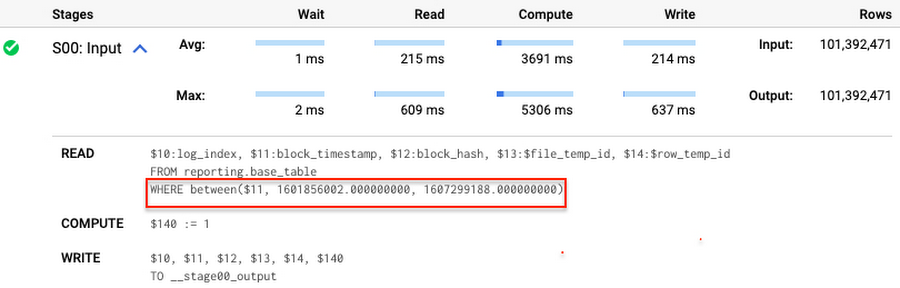
Note that you add the static filter to the staging table and keep T.block_timestamp = S.block_timestamp to convey to BigQuery that it can push that filter to the base table. This MERGE processes 41 GB of data in contrast to the initial 161 GB. You can see in the query plan that BigQuery pushes the partition filter from the staging table to the base table:
This type of optimization, when a pruning condition is pushed from a subquery to a large partitioned or clustered table, is not unique for MERGE. It also works for other types of queries. For instance:
SELECT * -- 41 GB processedFROM reporting.base_table TINNER JOIN staging.load_delta SON T.block_hash = S.block_hashAND T.log_index = S.log_indexAND T.block_timestamp = S.block_timestampWHERE S.block_timestamp BETWEEN TIMESTAMP '2020-10-05' AND TIMESTAMP '2020-12-07'
And you can check the query plan to verify that BigQuery pushed down the partition filter from one table to another.
Moreover, for SELECT statements, BigQuery can automatically infer a filter predicate on a join column and push it down from one table to another if your query meets the following criteria:
- The target table must be clustered or partitioned.
- The result size of the other table, i.e. after applying all filters, must qualify for broadcast join. Namly, the result set must be relatively small, less than ~100MB.
In our running example, reporting.base_table is partitioned by block_timestamp. If you define a selective filter on staging.load_delta and join two tables, you can see an inferred filter on the join key pushed to the target table
SELECT *FROM reporting.base_table TINNER JOIN staging.load_delta SON T.block_timestamp = S.block_timestampWHERE S.block_hash = '0x0c1caa16b34d94843aabfebc0d5a961db358135988f7498a6fdc450ad55f0870'
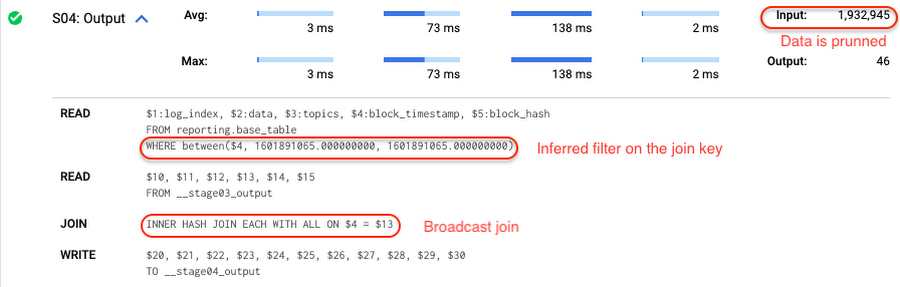
There is no requirement to join tables by partitioning or clustering key to kick off this type of optimization. However, in this case the pruning effect on the target table would be less significant.
But let us get back to the pipeline optimizations. Another way to enhance MERGE is to modify the merge_condition filter by adding static predicate on the base table:
BEGINDECLARE src_range STRUCT<date_min TIMESTAMP, date_max TIMESTAMP> --115 MB processedDEFAULT(SELECT STRUCT(MIN(block_timestamp) AS date_min,MAX(block_timestamp) AS date_max) FROM staging.load_delta);MERGE INTO reporting.base_table T --41 GB processedUSING staging.load_delta SON T.block_hash = S.block_hashAND T.log_index = S.log_indexAND T.block_timestamp BETWEEN src_range.date_min AND src_range.date_maxWHEN MATCHED THEN UPDATE SETT.data = S.dataWHEN NOT MATCHED THEN INSERT (log_index, data, topics, block_timestamp, block_hash)VALUES (log_index, data, topics, block_timestamp, block_hash);END;
To summarize, here are the steps that you can perform to enhance incremental ingestion pipelines in BigQuery. First you compute the range of updated partitions based on the small staging table. Next, you tweak the MERGE statement a bit to let BigQuery know to prune data in the base table.
All the enhanced MERGE statements scanned 41 GB of data, and setting up the src_range variable took 115 MB. Compare it with the initial 161 GB scan. Moreover, given that computing src_range may be incorporated into some existing transformation in your ETL/ELT, it results in a good performance improvement which you can leverage in your pipelines.
In this post we described how to enhance data ingestion pipelines by turning dynamic filter predicates into static predicates and letting BiQuery prune data for us. You can find more tips on BigQuery DML tuning here.
Special thanks to Daniel De Leo, who helped with examples and provided valuable feedback on this content.
Query Insights for Spanner: A blessing for developers and DBAs

3289
Of your peers have already read this article.
1:30 Minutes
The most insightful time you'll spend today!
Today, application development teams are more agile and are shipping features faster than ever before. In addition to these rapid development cycles and the rise of microservices architectures, the end-to-end ownership of feature development (and performance monitoring) has moved to a shared responsibility model between advanced database administrators and full-stack developers. However, most developers don’t have the years of experience or the time needed to debug complex query performance issues and database administrators are now a scarce resource in most organizations. As a result, there is a dire need for tools for developers and DBAs alike to quickly diagnose performance issues.
Introducing Query Insights for Spanner
We are delighted to announce the launch of Query Insights for Spanner, a set of visualization tools that provide an easy way for developers and database administrators to quickly diagnose query performance issues on Spanner. Using Query Insights, users can now troubleshoot query performance in a self-serve way. We’ve designed Query Insights using familiar design patterns with world-class visualizations to provide an intuitive experience for anyone who is debugging issues with query performance on Spanner. Query Insights is available at no additional cost.
By using out-of-the-box visual dashboards and graphs, developers can visualize aberrant behavior like peaks and troughs in various performance metrics over a time-series and quickly identify problematic queries. Time series data provides significant value to organizations because it enables them to analyze important real-time and historical metrics. Data is valuable only if it’s easy to comprehend;. that’s where being able to view intuitive dashboards becomes a force multiplier for organizations looking to expose their time series data across teams.
Follow a visual journey with pre-built dashboards
With Query Insights, developers can seamlessly move from detection of database performance issues to diagnosis of problematic queries using a single interface. Query Insights will help identify query performance issues easily with pre-built dashboards.
The user could do this by following a simple journey where they can quickly confirm, identify and analyze query performance issues. Let’s walk through an example scenario.
Understand database performance
This journey will start by the user setting up an alert on Google Cloud Monitoring for CPU utilization going above a certain threshold. The alert could be configured in a way that if this threshold is crossed, the user will be notified with an email alert, with a link to the “Monitoring” dashboard.
Once the user receives this alert, they would click on the link in the email, and navigate to the “Monitoring” dashboard. If they observe high CPU Utilization and high read latencies, the possible root cause could be expensive queries. A spike in CPU Utilization could be a strong signal that the system is using more compute than it usually would, due to an inefficient query.
The next step is to identify which query might be the problem, this is where Query Insights comes in. The user can get to this tool by clicking on Query Insights in the left navigation of your Spanner Instance. Here, they can drill down into the CPU usage by query and observe that for a specific database, CPU Utilization (attributed to all queries) is spiking for a particular time window. This confirms that the CPU utilization is due to inefficient queries.
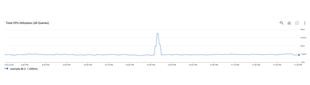
Identifying a problematic query
The user now observes the TopN (Top queries by CPU Utilization) query graph to see the TopN queries by CPU Utilization. From the graph, it is very easy to visualize and identify the top queries which could be causing the spike in CPU Utilization.
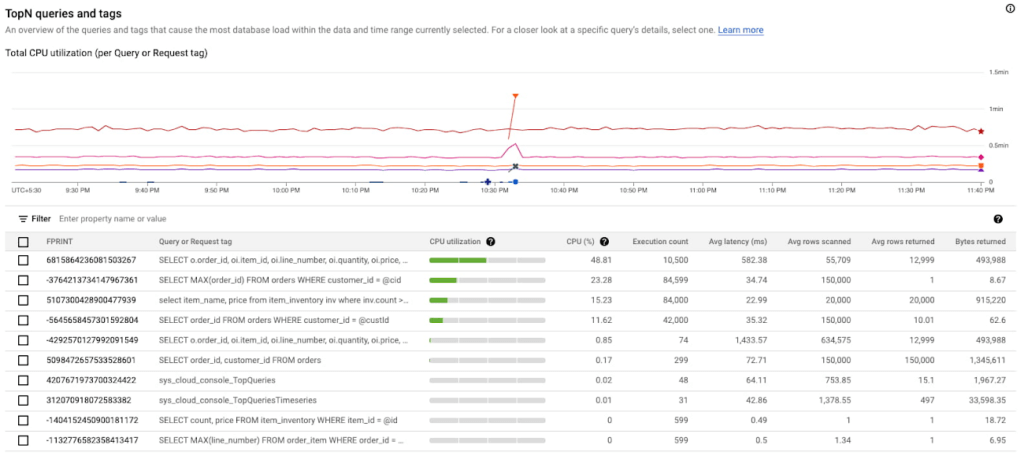
In the above screenshot, we can see that the first query in the table is showing a clear spike at 10:33 PM consuming 48.81% of total CPU. This is a clear indication that this query could be problematic, and the user should investigate further.
Analyzing the query performance
Once they have identified the problematic query, they can now drill down into this query shape to confirm, identify the root cause of the high CPU utilization.
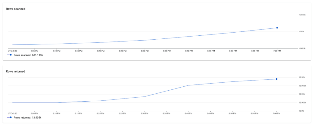
They can do this by clicking on the Fingerprint ID for the specific query from the topN table, and navigating to the Query Details page where they will be able to see a list of metrics (Latency, CPU Utilization, Execution count, Rows Scanned / Rows Returned) over a time series for that specific query.
In this example, we notice that the average number of rows scanned for this specific query are very high (~ 600k rows scanned to return ~ 12k rows), which could point to a poor query design, resulting in an inefficient query. We can also observe that latency is high (1.4s) for this query.
Fixing the issue
To fix the problem in this scenario, the user could optimize this query by specifying a secondary index in the query using a FORCE_INDEX query hint to provide an index directive. This would provide more consistent performance, make the query more efficient, and lower CPU utilization for this query.
In the screenshot below, you can see that after specifying the index in the query, the query performance dramatically increases in terms of CPU, rows scanned (54K vs 630k) and also in terms of query latency (536 ns vs 1.4 s).
Unoptimized Query:
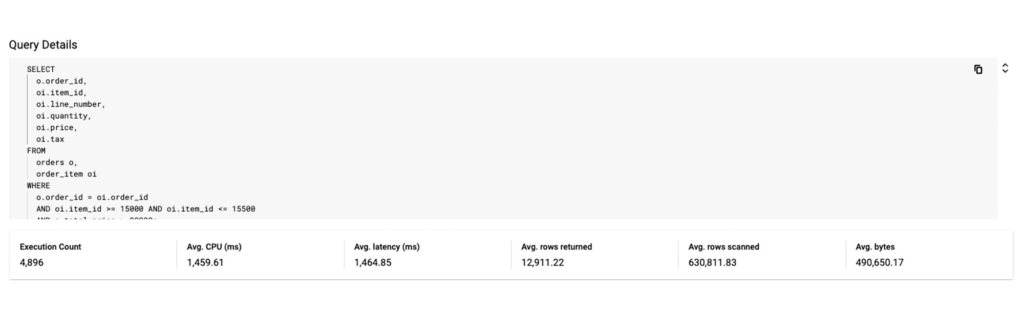
Optimized Query:
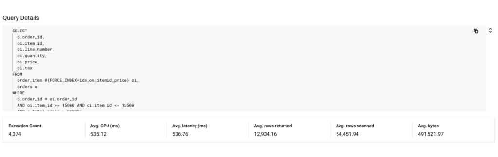
By following this simple visual journey, the user can easily detect, diagnose and debug inefficient queries on Spanner.
Get started with Query Insights today
To learn more about Query Insights, review the documentation here. Query Insights is enabled by default. In the Spanner console, you can click on Query Insights in the left navigation and start visualizing your query performance metrics!
New to Spanner? Get started in minutes with a new database.
Home Depot Leverages Google Cloud’s BigQuery and DataFlow to Break Data Silos and Craft Personalized CX

4989
Of your peers have already read this article.
4:00 Minutes
The most insightful time you'll spend today!
The Home Depot, Inc., is the world’s largest home improvement retailer with annual revenue of over $151B. Delighting our customers—whether do-it-yourselfers or professionals—by providing the home improvement products, services, and equipment rentals they need, when they need them, is key to our success.
We operate more than 2,300 stores throughout the United States, Canada, and Mexico. We also have a substantial online presence through HomeDepot.com, which is one of the largest e-commerce platforms in the world in terms of revenue. The site has experienced significant growth both in traffic and revenue since the onset of Covid-19.
Because many of our customers shop at both our brick-and-mortar stores and online, we’ve embarked on a multi-year strategy to offer a shopping experience that seamlessly bridges the physical and digital worlds. To maximize value for the increasing number of online shoppers, we’ve shifted our focus from event marketing to personalized marketing, as we found it to be far more effective in improving the customer experience throughout the sales journey. This led to changing our approach to marketing content, email communications, product recommendations, and the overall website experience.
Challenge: launching a modern marketing strategy using legacy IT
For personalized marketing to be successful, we had to improve our ability to recognize a customer at the point of transaction so we could—among other things—suspend irrelevant and unnecessary advertising. Most of us have experienced the annoyance of receiving ads for something we’ve already purchased, which can degrade our perception of the brand itself. While many online retailers can identify 100% of their customer transactions due to the rich information captured during checkout, most of our transactions flow through physical stores, making this a more difficult problem to solve.
Our old legacy IT system, which ran in an on-premises data center and leveraged Hadoop, also challenged us since maintaining both the hardware and software stack required significant resources. When that system was built, personalized marketing was not a priority, so it took several days to process customer transaction data and several weeks to roll out any system changes. Further, managing and maintaining the large Hadoop cluster base presented its own set of issues in terms of quality control and reliability, as did keeping up with open-source community updates for each data processing layer.
Adopting a hybrid approach
As we worked through the challenges of our legacy system, we started thinking about what we wanted our future system to look like. Like many companies, we began with a “build vs. buy” analysis. We looked at several products on the market and determined that while each of them had their strengths, none was able to offer the complete set of features we needed.
Our project team didn’t think it made sense to build a solution from scratch, nor did we have access to the third-party data we needed. After much consideration, we decided to adopt a solution that combined a complete rewrite of the legacy system with the support of a partner to help with the customer transaction matching process.
Building the foundation on Google Cloud
We chose Google Cloud’s data platform, specifically BigQuery, Dataflow, DataProc, Cloud Storage, and Cloud Composer. Google Cloud platform empowered us to break down data silos and unify each stage of the data lifecycle from ingestion, storage, and processing to analysis and insights. Google Cloud offered best-in-class integration with open-source standards and provided the portability and extensibility we needed to make our hybrid solution work well. The open standards of BigQuery’s BQ Storage API allowed us to leverage fast BQ storage layers to be utilized with other compute platforms, e.g., DataProc.
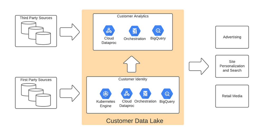
We used BigQuery combined with Dataflow to integrate our first- and third-party data into an enterprise data and analytics data lake architecture. The system then combined previously siloed data and used BigQuery ML to create complete customer profiles spanning the entire shopping experience, both in-store and online.
Understanding the customer journey with the help of Dataflow and BigQuery
The process of developing customer profiles involves aggregating a number of first- and third-party data sources to create a 360-degree view of the customer based on both their history and intent. It starts with creating a single historical customer profile through data aggregation, deduplication, and enrichment. We used several vendors to help with customer resolution and NCOA (Change of Address) updates, which allows the profile to be house-holded and transactions to be properly reconciled to both the individual and the household. This output is then matched to different customer signals to help create an understanding of where the customer is in their journey—and how we can help.
The initial implementation used Google Dataflow, Google’s streaming analytics solution, to load data from Google Cloud Storage into BigQuery and perform all necessary transformations. The Dataflow process was converted into BQML (BigQuery Machine Learning) since this significantly reduced costs and increased visibility into data jobs. We used Google Cloud Composer, a fully managed workflow orchestration service, to help orchestrate all data operations and DataProc and Google Kubernetes Engine to enable special case data integration so we could quickly pivot and test new campaigns. The architecture diagram below shows the overall structure of our solution.
Taking full advantage of cloud-native technology
In our initial migration to Google Cloud, we moved most of our legacy processes in their original form. However, we quickly learned that this approach didn’t take full advantage of the cloud-native and more improved features Google Cloud offered such as auto scaling of resources, flexibility to decouple storage from the compute layer, and a wide variety of options to choose the best tool for the job. We refactored our Hadoop-based data pipelines written in Java-based Map Reduce and our Pig Latin jobs to Dataflow and BigQuery jobs. This dramatically reduced processing time and made our data pipeline code concise and efficient.
Previously, our legacy system processes ran longer than intended, and data was not used efficiently. Optimizing our code to be cloud-native and leveraging all the capabilities of Google Cloud services resulted in reduced run times. We decreased our data processing window from 3 days to 24 hours, improved resource usage by dramatically reducing the amount of compute we used to possess this data, and built a more streamlined system. This in turn reduced cloud costs and provided better insight. For example, DataFlow offers powerful native features to monitor data pipelines, enabling us to be more agile.
Leveraging the flexibility and speed of the cloud to improve outcomes
Today, using a continuous integration/continuous delivery (CI/CD) approach, we can deploy multiple system changes each week to further improve our ability to recognize in-store transactions. Leveraging the combined capabilities of various Google Cloud systems—BigQuery, DataFlow, Cloud Composer, Dataproc, and Cloud Storage–we drastically increased our ability to recognize transactions and can now connect over 75% of all transactions to an existing household. Further, the flexible Google Cloud environment coupled with our cloud-native application makes our team more nimble and better able to respond to emerging problems or new opportunities.
Increased speed has led to better outcomes in our ability to match transactions across all sales channels to a customer and thereby improve their experience. Before moving to Google Cloud, it took 48 to 72 hours to match customers to their transactions, but now we can do it in less than 24 hours.
Making marketing more personal—and more efficient
The ability to quickly match customers to transactions has huge implications for our downstream marketing efforts in terms of both cost and effectiveness. By knowing what a customer has purchased, we can turn off ads for products they’ve already bought or offer ads for things that support what they’ve bought recently. This helps us use our marketing dollars much more efficiently and offer an improved customer experience.
Additionally, we can now apply the analytical models developed using BQML and Vertex AI to sort customers into audiences. This allows us to more quickly identify a customer’s current project, such as remodeling a kitchen or finishing a basement, and then personalize their journey by offering them information on products and services that matter most at a given point through our various marketing channels. This provides customers with a more relevant and customized shopping journey that mirrors their individual needs.
Protecting a customer’s privacy
With this ability to better understand our customers, we also have the responsibility to ensure we have good oversight and maintain their data privacy. Google’s cloud solutions provide us the security needed to help protect our customers’ data, while also being flexible enough to allow us to support state and federal regulations, like the California Customer Privacy Act. This way we can provide a customer the personalized experience they desire without having to fear how their data is being used.
With flexible Google Cloud technology in place, The Home Depot is well positioned to compete in an industry where customers have many choices. By putting our customers’ needs first, we can stay top of mind whenever the next project comes up.
Google Cloud Announces General Availability of BigQuery Row-level Security
6589
Of your peers have already read this article.
3:00 Minutes
The most insightful time you'll spend today!
Data security is an ongoing concern for anyone managing a data warehouse. Organizations need to control access to data, down to the granular level, for secure access to data both internally and externally. With the complexity of data platforms increasing day by day, it’s become even more critical to identify and monitor access to sensitive data. In many cases, sensitive data is co-mingled with non-sensitive data, and access restrictions to sensitive data need to be enabled based on factors like data location or presence of financial information. There may also be nuances where data is sensitive for some groups of users, while for others, it is not.
Today, we’re pleased to announce the general availability of BigQuery row-level security, which gives customers a way to control access to subsets of data in the same table for different groups of users. Row-level security (RLS) extends the principle of least privilege access and enables fine-grained access control policies in BigQuery tables. BigQuery currently supports access controls at the project-, dataset-, table- and column-level. Adding RLS to the portfolio of access controls now enables customers to filter and define access to specific rows in a table based on qualifying user conditions—providing much needed peace of mind for data professionals.
“Our digital transformation and migration of data to the cloud magnifies the business value we can extract from our information assets. However, granular data access control is essential to comply with international regulatory and contractual requirements. BigQuery row-level security helps us comply with data residency and export restrictions,” says Jarrett Garcia, Iron Mountain’s Enterprise Data Platform Senior Director. “It enables us to manage fine-grained access controls without replicating data. What used to take months for approval and access provisioning can now be done more efficiently and effectively. We are looking forward to implementing additional data security capabilities on the BigQuery roadmap to address other critical business use cases.”
How BigQuery row-level security works
Row-level security in BigQuery enables different user personas access to subsets of data in the same table. Customers who are currently using authorized views to enable these use cases can leverage RLS for ease of management. To express the concept of RLS, we have introduced a new entity in BigQuery called row access policy. Row access policies map a group of user principals to the rows that they can see, defined by a SQL filter predicate.
Secure logic rules created by data owners and administrators determines which user can see which rows through the creation of a row-level access policy. The row-level access policies created on a target table by administrators or data owners are applied when a query is run on the table. One table can have multiple policies applied to it.
Below is an example, where row-level access policies have been created to filter data based on users’ “region”.

In the illustrated scenario above, row-level access policies have been created to verify a querying user’s region and to give them access only to the subset of data relevant to that region. Access policies are granted to a grantee list which support all types of IAM principles such as individual users, groups, domains or service accounts. In this example, when a user queries the table, row-level access policies are evaluated to assess which, if any, policies are applicable to that user. The group ‘sales-apac’ is granted access to view a subset of rows where region = ‘APAC’ whereas the group ‘sales-us’ is granted access to view a subset of rows where the region = ’US’. Likewise, users in both groups will see rows in both regions, and users in neither group will not see any rows.
Row-level access policies can also be created using the SESSION_USER() function to restrict access only to rows that belong to the user running the query. If none of the row access policies are applicable to the querying user, the user will have no access to the data in the table.
When a user queries a table with a row-level access policy, BigQuery displays a banner notice indicating that their results may be filtered by a row-level access policy. This notice displays even if the user is a member of the `grantee_list`.

When to put BigQuery row-level security to work
Row-level access policies are useful when you have a need to limit access to data based on filter conditions. The row-access policies’ filter predicate supports arbitrary SQL, and is conceptually similar to the WHERE clause of a SQL query. Filter predicates support the SESSION_USER() function to restrict access only to rows that belong to the user running the query. If none of the row access policies are applicable to the querying user, the user will have no access to the data in the table. Currently, the column used for filtering must be in the table, but we anticipate adding support for subqueries in the filter expression, opening up access to use cases where data is filtered based on lookup tables and calculated values. Row-level access policies can be created, updated and dropped using DDL statements. You will be able to see the list of row-level access policies applied to a table using the BigQuery schema pane in the Cloud Console, which simplifies the management of policies per table, or by using the bq command-line tool.
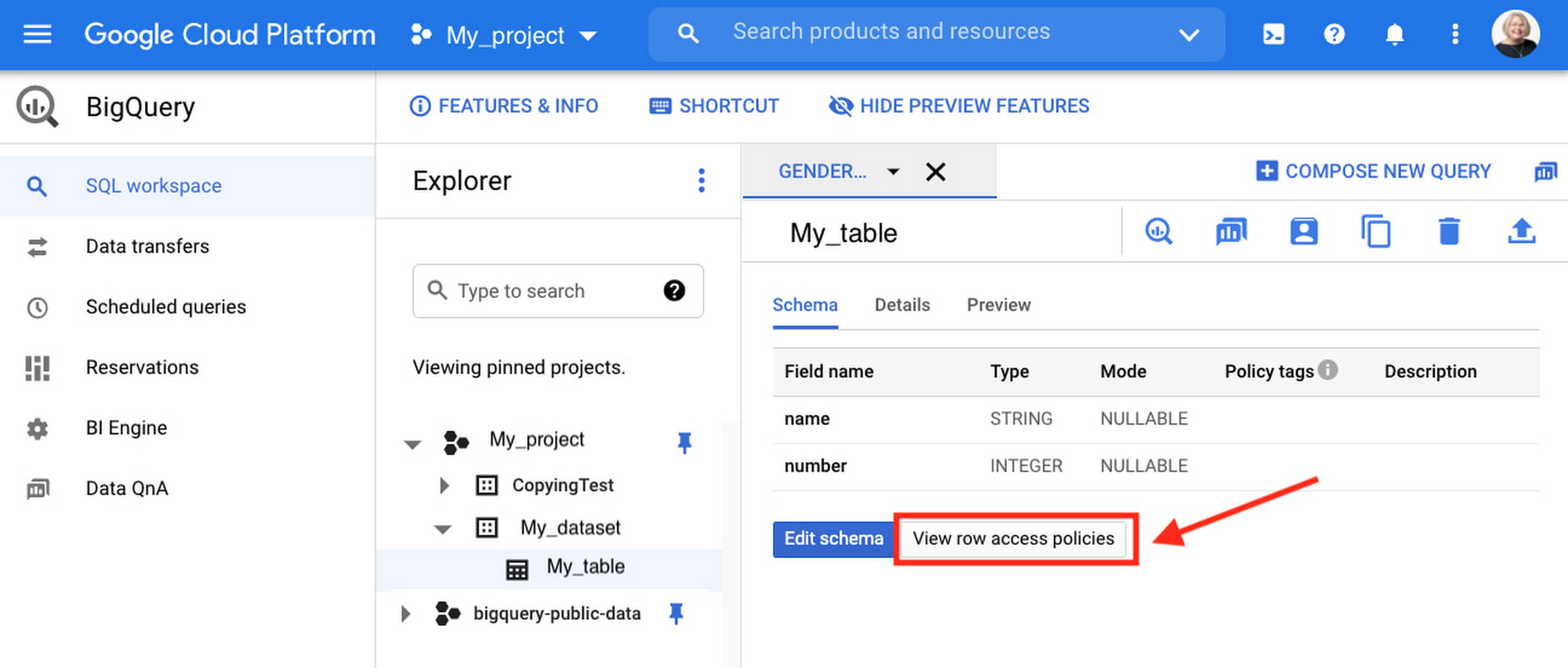
Row-level security is compatible with other BigQuery security features, and can be used along with column-level security for further granularity. Since row-level access policies are applied on the source tables, any actions performed on the table will inherit the table’s associated access policies, to ensure access to secure data is protected. Row-level access policies are applicable to every method used to access BigQuery data (API, Views, etc).
Try it out
We’re always working to enhance BigQuery’s (and Google Cloud’s) data governance capabilities, to provide more controls around managing your data. With row-level security, we are adding deeper protections for your data. You can learn more about BigQuery row-level security in our documentation and best practices.
More Relevant Stories for Your Company

Serverless and BigQuery Together on Google Cloud: Behind the L’Oreal Beauty Tech Data Platform
Editor's note: In Today's guest post we hear from beauty leader L'Oréal about their approach to building a modern data platform on fully managed services: managing the ingest of diverse datasets into BigQuery with Cloud Run, and orchestrating transformations into relevant business domain representations for stakeholders across the organization. Learn


Can Your Data Warehouse Handle a 100-Trillion Row Query?
Today's enterprise demands from data go far beyond the capabilities of traditional data warehousing and for many leaders, the need to digitally transform their businesses is a key driver for data analytics spending. Businesses want to make real-time decisions from fresh information as well as make future predictions from their

Two Ad Agencies Leverage BigQuery to Support Next-gen Ad Campaigns
Advertising agencies are faced with the challenge of providing the precision data that marketers require to make better decisions at a time when customers’ digital footprints are rapidly changing. They need to transform customer information and real-time data into actionable insights to inform clients what to execute to ensure the

Want to Code for the Cloud? Get Started with the Native App Development Track
Earlier this year, we launched the Google Cloud skills challenge, which provides 30 days of free access to training to build your cloud knowledge and an opportunity to earn skill badges that showcase your Google Cloud competencies. Today, we’re adding a Native App Development track to the skills challenge, joining the Getting Started,
