





Boost Database Performance with AlloyDB Index Advisor: The Ultimate Optimization Tool

1378
Of your peers have already read this article.
4:00 Minutes
The most insightful time you'll spend today!
Intro
One of the time consuming tasks for DBAs is to maximize query performance. To optimize slow-running queries, they often have to do detailed analysis, understand optimizer plans, and go through a lot of trial and error before getting to the best set of indexes that help with improved query performance. However, even with expert knowledge of a database’s internals, it is challenging to choose an effective set of indexes, especially when workloads change over time. The complexity of queries including several joins, filters, and subqueries make the process of identifying the right set of indexes very challenging for DBAs. Also, the effect of an index on the query plan needs to be taken into account when considering further indexes. Creating an index may cause the query optimizer to select completely different join orders and join/scan methods. This effect is hard to predict and quantify for DBAs.
Imagine if the database itself is intelligent enough to identify such queries, and recommends creating specific B-tree indexes?
Google Cloud’s AlloyDB for PostgreSQL is a fully-managed and fully PostgreSQL-compatible database for demanding transactional and analytical workloads that provides enterprise-grade performance and availability. AlloyDB offers Index Advisor, a built-in feature that helps alleviate the guesswork of tuning query performance with deep analysis of the different parts of a query including subqueries, joins, and filters. It periodically analyzes the database workload, identifies queries that can benefit from indexes, and recommends new indexes that can increase query performance.
How the AlloyDB Index Advisor works
First, let’s review a few AlloyDB terms relevant to the Index Advisor’s work.
- PostgreSQL’s system catalog has schema metadata, such as information about tables and columns, and internal bookkeeping information.
- HypoPG is an open source PostgreSQL extension that helps with hypothetical indexes without actually creating them to see if the index helps with query execution.
- Query Optimizer generates optimal execution plan.
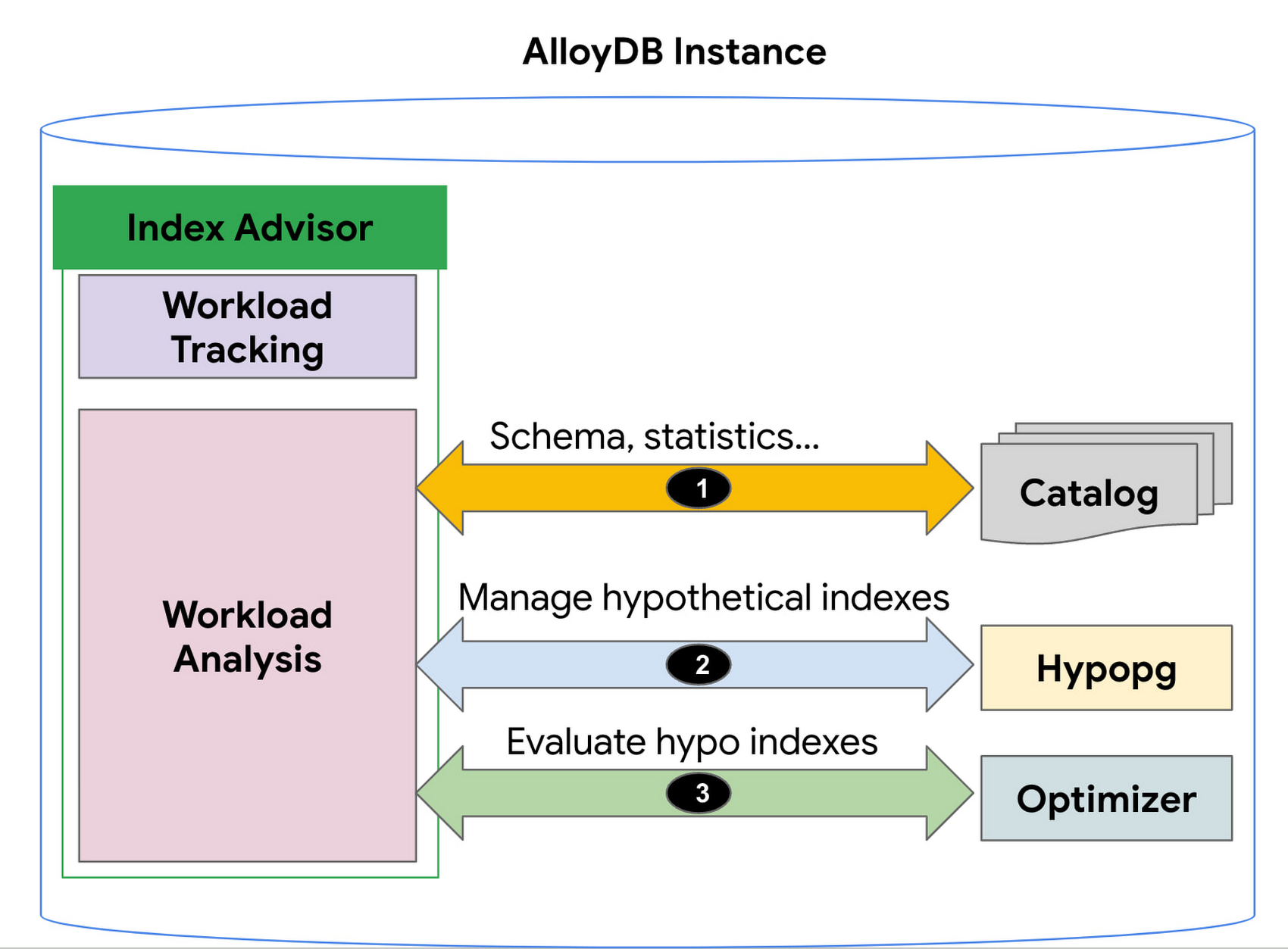
1. AlloyDB’s Index Advisor tracks the user query workload and analyzes it using statistics from the system catalog; it then identifies queries that could be improved significantly and potential candidate indexes for those cases. Note that there could be a large number of candidate indexes.
2. The Index Advisor evaluates each of these queries using hypothetical indexes based on the HypoPG, an open source extension and AlloyDB’s Query Optimizer.
3. The results of this evaluation are used to intelligently select the best set of indexes for the workload and to generate recommendations.
You can then simply copy and run the suggested index creation SQL commands. The Index Advisor consumes minimal resources and analyzes queries at a frequency that you define. It can also be constrained to have a user-specified maximum storage budget for the new indexes it recommends.
How to use the Index Advisor
1. Index Advisor is enabled by default. Its recommendation engine analyzes your workload at the specified frequency (every 24 hours by default) to capture any potential new index recommendations.
2. Run your queries that are representative of your workload to the instance. Index advisor tracks these queries automatically.
3. To request an index recommendation immediately, you can use the google_db_advisor_recommend_indexes() function. This function performs on-demand analysis and recommends indexes for the top 100 queries. SELECT * FROM google_db_advisor_recommend_indexes();
4. To view the recommended indexes and the queries based on periodic analysis, use the following query (also see the Usage Example section). SELECT DISTINCT recommended_indexes, queryFROM google_db_advisor_workload_report r JOIN google_db_advisor_workload_statements sON r.query_id = s.query_id;
Note that Index advisor analyzes queries issued by the connected user. For the user with the pg_read_all_stats role, it analyzes all tracked queries.
Currently, Index advisor only recommends new indexes. In future, the Index Advisor could be used to report unused indexes as well; dropping these can reduce index maintenance overhead for your transactional workload.
Evaluation
We will discuss two cases in this section.
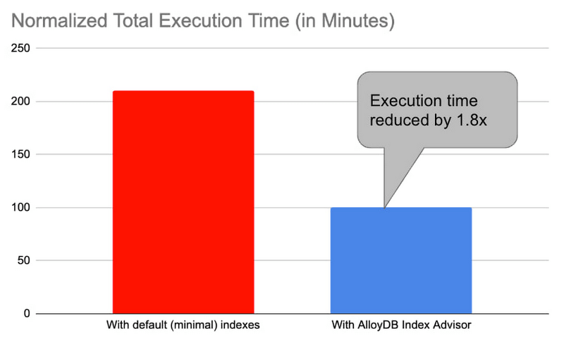
1. Decision support benchmark: We used a sample internal benchmark that modeled a decision support system. The benchmark dataset contained 450+ columns across 24 tables. The result quantified the performance of 100+ complex analytical queries. The benchmark initially had a minimal number of indexes and the normalized total query execution time was around 200+ minutes. We then enabled the AlloyDB Index Advisor and it recommended an additional 17 indexes. Creating those indexes and re-running the queries reduced the total execution time by half to ~100 minutes (1.8x).
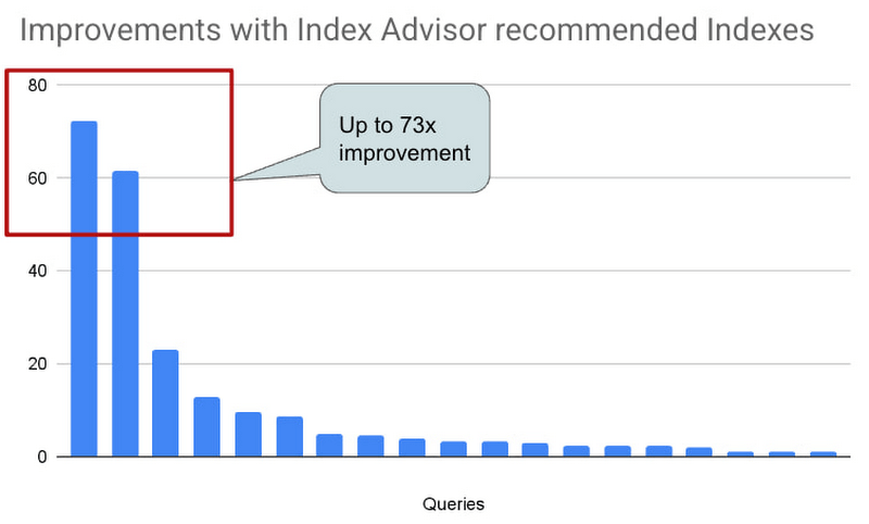
2. Real-world AlloyDB customer workload: This is a real-world workload from a large financial customer. They have a portfolio of complex analytical queries and business insights demand fast response times. Before using Index Advisor, DBAs had already created a few indexes that they considered to be useful to speed up these queries. Many of their queries joined 30+ tables, had 10+ filters and multiple subqueries. Those made it complex for DBAs to correctly identify the most beneficial indexes to create. AlloyDB Index Advisor analyzed these complex structures and identified four additional indexes. By adding the suggested indexes, performance of 17 queries were up by 5x – 73x. The response time of these queries dropped from seconds to milliseconds.
Usage Example
An example: We use the following example to demonstrate the use of Index Advisor. The example simulates a retail application performing analytics on its orders table.
1. Create a sample orders table.
CREATE TABLE orders (
    o_orderkey bigint NOT NULL,
    o_custkey int NOT NULL,
    o_orderstatus "char" NOT NULL,
    o_totalprice numeric(13,2) NOT NULL,
    o_orderdate date NOT NULL,
    o_orderpriority character varying(15) NOT NULL,
    o_clerk character varying(15) NOT NULL,
    o_shippriority int NOT NULL,
    o_comment character varying(79) NOT NULL
);
2. Insert 100K random orders into the table.
INSERT INTO orders
SELECT col, col, substr(md5(random()::text), 1, 1), random(), date '2023-01-01' + col * interval '1 hour', substr(md5(random()::text), 1, 1), concat('clerk', col), col%10, concat('comment', col)
 FROM generate_series(1,1000000) g(col);
3. Analyze the table to populate statistics.
ANALYZE orders;4. Run a query that counts the number of orders in the second week of Jan. You can run the query with timing on so that you can see how long it takes to run the query before and after the index is created.
\timing
SELECT COUNT(*) FROM ORDERS WHERE o_orderdate >= '2023-01-09' and o_orderdate <= '2023-01-15';

Time: 42.196 ms
5. Manually request an index recommendation.
SELECT * FROM google_db_advisor_recommend_indexes();
                      index                       | estimated_storage_size_in_mb
--------------------------------------------------+------------------------------
 CREATE INDEX ON "public"."orders"("o_orderdate") |                           25
(1 row)
6. View recommended indexes for tracked queries.
SELECT DISTINCT recommended_indexes, query
FROM google_db_advisor_workload_report r, google_db_advisor_workload_statements s
WHERE r.query_id = s.query_id AND recommended_indexes != '';
               recommended_indexes                |                                             query
--------------------------------------------------+------------------------------------------------------------------------------------------------
 CREATE INDEX ON "public"."orders"("o_orderdate") | SELECT COUNT(*) FROM ORDERS WHERE o_orderdate >= '2023-01-09' and o_orderdate <= '2023-01-15';
(1 row)
6. View recommended indexes for tracked queries.
SELECT DISTINCT recommended_indexes, query
FROM google_db_advisor_workload_report r, google_db_advisor_workload_statements s
WHERE r.query_id = s.query_id AND recommended_indexes != ”;
recommended_indexes | query
————————————————–+————————————————————————————————
CREATE INDEX ON “public”.”orders”(“o_orderdate”) | SELECT COUNT(*) FROM ORDERS WHERE o_orderdate >= ‘2023-01-09’ and o_orderdate <= ‘2023-01-15’;
(1 row)
7. Add the recommended index.
CREATE INDEX ON "public"."orders"("o_orderdate");8. Re-run the query.
\timing
SELECT COUNT(*) FROM ORDERS WHERE o_orderdate >= '2023-01-09' and o_orderdate <= '2023-01-15';

Time: 1.403 ms  (compared to 42.196ms before the index)
Learn more
- To learn more about AlloyDB’s Index Advisor, see Enable and use the index advisor | AlloyDB for PostgreSQL | Google Cloud
- To learn about AlloyDB, read AlloyDB for PostgreSQL intelligent scalable storage | Google Cloud Blog
- Start building on Google Cloud with $300 in free credits and 20+ always free products. https://cloud.google.com/free
Google Launches Open Saves To Power Gaming Platforms Scale to User Demands

5482
Of your peers have already read this article.
1:30 Minutes
The most insightful time you'll spend today!
Many of today’s games are rich, immersive worlds that engage the audience in ways that make a gamer a part of a continuing storyline. To create these persistent experiences, numerous storage technologies are required to ensure game data can scale to the standards of gamers’ demands. Not only do game developers need to store different types of data—such as saves, inventory, patches, replays, and more—but they also must keep the storage system high-performing, available, scalable, and cost-effective.
Enter Open Saves, a brand-new, purpose-built single interface for multiple storage back ends that’s powered by Google Cloud and developed in partnership with 2K. Now, development teams can store game data without having to make the technical decisions on which storage solution to use, whether that’s Cloud Storage, Memorystore, or Firestore.
“Open Saves demonstrates our commitment to partnering with top developers on gaming solutions that require a combination of deep industry expertise and Google scale,” said Joe Garfola, Vice President of IT and Security at 2K. “We look forward to continued collaboration with Google Cloud.”
Game development teams can save game data against Open Saves without having to worry about the optimal back-end storage solution, while operations teams can focus on needed scalability and storage options. Here’s how it looks in practice:
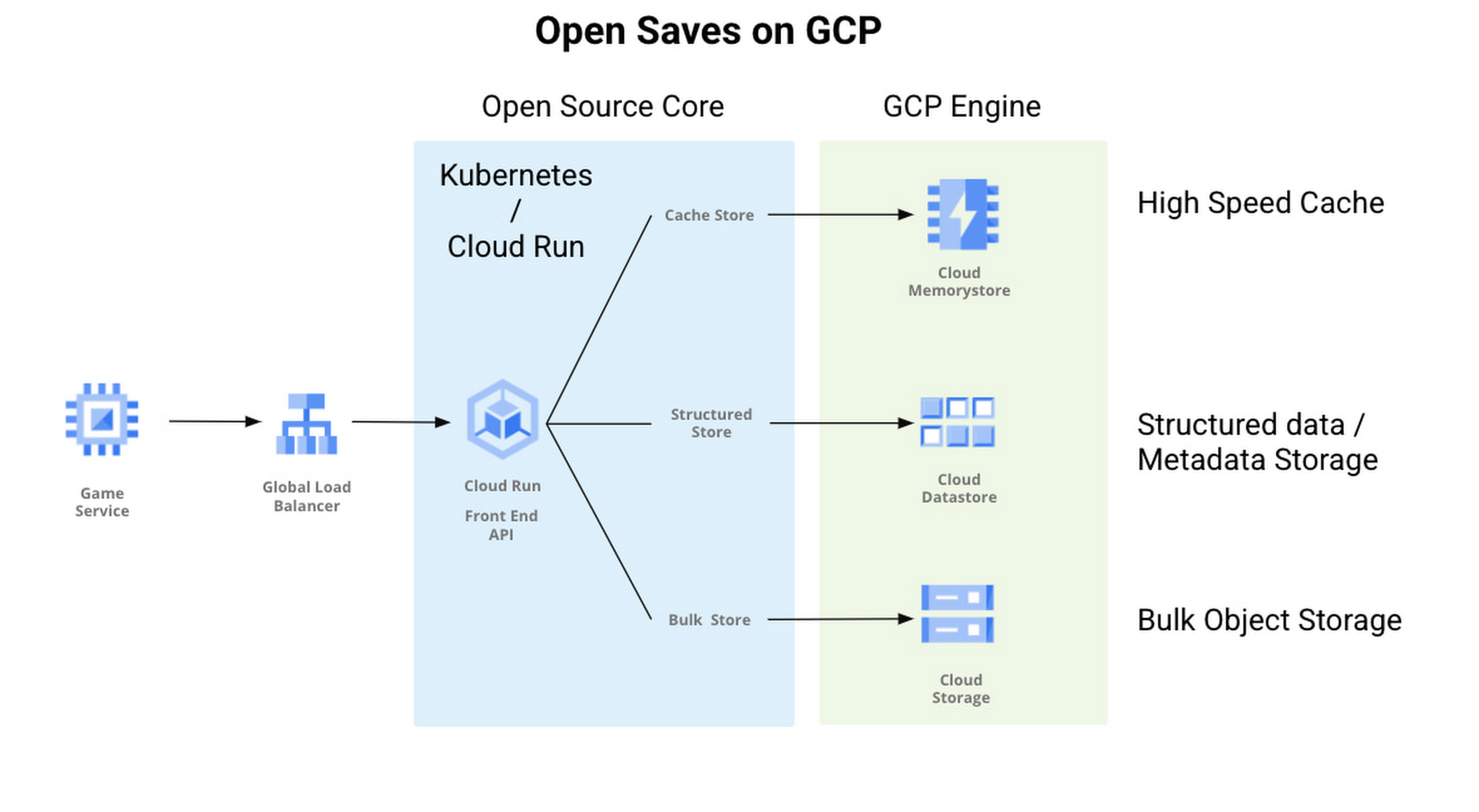
With Open Saves, game developers can run a cloud-native game storage system that is:
- Simple: Open Saves provides a unified, well-defined gRPC endpoint for all operations for metadata, structured, and unstructured objects.
- Fast: With a built-in caching system, Open Saves optimizes data placements based on access frequency and data size, all to achieve both low latency for smaller binary objects and high throughput for big objects.
- Scalable: The Open Saves API server can run on either Google Kubernetes Engine or Cloud Run. Both platforms can scale out to handle hundreds of thousands of requests per second. Open Saves also stores data in Firestore and Cloud Storage, and can handle hundreds of gigabytes of data and up to millions of requests per second.
Open Saves is designed with extensibility in mind, and can be integrated into any game—whether mobile or console, multiplayer or single player—running on any infrastructure, from on-prem to cloud or a hybrid. The server is written in Go, but you can use many programming languages and connect from client or server since the API is defined in gRPC.
Writing to and reading from Open Saves is as simple as the following code:
// To writerecord := &pb.Record{Key: uuid.New().String(),Tags: []string{"tag1", "tag2"},OwnerId: "owner",}createReq := &pb.CreateRecordRequest{StoreKey: storeKey,Record: record,}_, err := client.CreateRecord(ctx, createReq)if err != nil {t.Fatalf("CreateRecord failed: %v", err)}// To readgetReq := &pb.GetRecordRequest{StoreKey: storeKey, Key: recordKey}response, err := client.GetRecord(ctx, getReq)if err != nil {t.Errorf("GetRecord failed: %v", err)}
We are actively developing Open Saves in partnership with 2K Games, and would love for you to come join us on GitHub. There are a few ways to get involved:
- Install and deploy your Open Saves service
- Check out the API reference
- Read the development guide and start contributing
- Join the open-saves-discuss mailing list
How Data Teams in EdTech Firms Make Most of the Educational Data at All Levels

3539
Of your peers have already read this article.
1:30 Minutes
The most insightful time you'll spend today!
Education data can inform strategy, enhance both teaching and learning, and help us better understand customer needs. But that data is only as useful as an organization’s ability to access, analyze, and act upon it. Education Technology (EdTech) companies with a strong data warehouse management policy can help to make the most of educational data at all levels.
Creating a data team
When an EdTech doesn’t have a dedicated data team, databases will likely be poorly maintained and data can be hard to find, it can lack critical security, or fail to meet a customer’s specific requirements. A dedicated data team can prevent this and better support an organization’s data needs. There’s a correlation between the maturity of a data team and the success of an organization’s data utilization. When considering the three primary components of team, outlook, and results, we can better understand an organization’s maturity. By using this matrix from Looker’s Analytical Maturity Playbook, you can assess the maturity of your organization’s data team. Most would agree, the goal is for your operation to move from data chaos to data-driven. But, how can you do that? Think about your data this way: the intelligence you gain from your data is not only an asset…it’s a product. When your data team views your business intelligence as a product—one that’s just as important as the services you offer—they can set the stage for creating a successful data-driven company. Mature data organizations:
- Report functionality regularly
- Constantly assess potential improvements to existing systems
- Manage content rollout to internal employees
Redivis: Making data accessible, connected & secure
Redivis is a platform that connects academic researchers with data and the tools to understand education intelligence. Their customers, who are researchers, expressed how difficult it is to find new datasets for their studies. Once they found a dataset, they often had to access and work with it before they could tell if the information would be useful for their studies. Redivis Data administrators were also concerned about data security. Redivis built their platform on top of Google Cloud’s security infrastructure, making it a highly scalable data processing environment.
Redivis developed a transparent, tiered access system for datasets that allows researchers to request separate access to a dataset’s documentation to determine whether they can use the dataset. Detailed audit logs (supported by Google Cloud Logging) and robust application-level security controls tighten data access. To offer more insights for their researchers, they securely connected their private datasets with public datasets hosted in BigQuery allowing researchers to run queries on billions of records in seconds, not hours.
With a data team in place, it’s time to visualize where to store and organize your data. Data is an asset. You want to invest in collecting, operationalizing, and storing it properly. “Inadequate data aggregation, harmonization, and processing impedes teams from making the right data-driven decisions and pivoting when needed,” according to Jesus Trujillo Gomez, a strategic business executive at Google Cloud. You can determine how mature your warehouse is by using this matrix to help you identify where your organization falls on the spectrum (least mature on the left, most mature on the right). A company’s data warehouse can be assessed in four areas: Technology, Pipeline, Quality, and Performance. Here are some suggested steps to bring your EdTech company one step closer to a data powerhouse.
Classcraft: Using a data-driven approach to make learning fun
Launched in 2014, learning company Classcraft is reimagining the classroom, creating better learning environments with gamification. To support their mission, their team has created a complete data platform that uses data analytics to find new ways to engage students in the classroom. Classcraft became a Google for Education Build Partner to keep up with rising demand. They expanded their footprint to reach 6 million students and educators in 165 countries.
They also migrated to Google Cloud, building on several integrations with Google Workspace for Education, Google Classroom, and Chrome for Education, allowing them to support customers ranging from individual teachers to entire school districts. Classcraft migrated its database and analytics infrastructure to BigQuery and Cloud Storage. “We capture about 10 million new data points every month related to school culture and student performance,” says Chief Technology Officer and VP of Product Stéphane Guillemette. “With BigQuery and other Google Cloud tools, we can quickly deliver valuable insights to educators.”
6692
Of your peers have already downloaded this article
4:30 Minutes
The most insightful time you'll spend today!
Unlocking the Power of Data and Creativity with
the Cloud: The WPP Story
How to Enhance Incremental Pipeline Performance while Ingesting Data into BigQuery

6308
Of your peers have already read this article.
3:00 Minutes
The most insightful time you'll spend today!
When you build a data warehouse, the important question is how to ingest data from the source system to the data warehouse. If the table is small you can fully reload a table on a regular basis, however, if the table is large a common technique is to perform incremental table updates. This post demonstrates how you can enhance incremental pipeline performance when you ingest data into BigQuery.
Setting up a standard incremental data ingestion pipeline
We will use the below example to illustrate a common ingestion pipeline that incrementally updates a data warehouse table. Let’s say that you ingest data into BigQuery from a large and frequently updated table in the source system, and you have Staging and Reporting areas (datasets) in BigQuery.

The Reporting area in BigQuery stores the most recent, full data that has been ingested from the source system tables. Usually you create the base table as a full snapshot of the source system table. In our running example, we use BigQuery public data as the source system and create reporting.base_table as shown below. In our example each row is identified by a unique key which consists of two columns: block_hash and log_index.
CREATE TABLE reporting.base_table --156 GB processedPARTITION BY TIMESTAMP_TRUNC(block_timestamp, DAY) ASSELECT log_index, data, topics, block_timestamp, block_hashFROM bigquery-public-data.crypto_ethereum.logsWHERE block_timestamp BETWEEN TIMESTAMP '2020-01-01' AND TIMESTAMP '2020-11-30';
In data warehouses it is common to partition a large base table by a datetime column that has a business meaning. For example, it may be a transaction timestamp, or datetime when some business event happened, etc. The idea is that data analysts who use the data warehouse usually need to analyze only some range of dates and rarely need the full data. In our example, we partition the base table by block_timestamp which comes from the source system.
After ingesting the initial snapshot you need to capture changes that happen in the source system table and update the reporting base table accordingly. This is when the Staging area comes into the picture. The staging table will contain captured data changes that you will merge into the base table. Let’s say that in our source system on a regular basis we have a set of new rows and also some updated records. In our example we mock the staging data as follows: first, we create new data, than we mock the updated records:
CREATE TABLE staging.load_delta AS --5 GB processedSELECT log_index, data, topics, block_timestamp, block_hashFROM bigquery-public-data.crypto_ethereum.logsWHERE block_timestamp BETWEEN TIMESTAMP '2020-12-01' AND TIMESTAMP '2020-12-07';INSERT INTO staging.load_delta --2 GB processedSELECT log_index, CONCAT(data, RAND()), topics, block_timestamp, block_hashFROM bigquery-public-data.crypto_ethereum.logs TABLESAMPLE SYSTEM (5 PERCENT)WHERE block_timestamp BETWEEN TIMESTAMP '2020-10-01' AND TIMESTAMP '2020-11-30';
Next, the pipeline merges the staging data into the base table. It joins two tables by unique key and than updates the changed value or inserts a new row
MERGE INTO reporting.base_table T --161 GB processedUSING staging.load_delta SON T.block_hash = S.block_hashAND T.log_index = S.log_indexWHEN MATCHED THEN UPDATE SETT.data = S.dataWHEN NOT MATCHED THEN INSERT (log_index, data, topics, block_timestamp, block_hash)VALUES (log_index, data, topics, block_timestamp, block_hash);
It is often the case that the staging table contains keys from various partitions but the number of those partitions are relatively small. It holds, for instance, because in the source system the recently added data may get changed due to some initial errors or ongoing processes but older records are rarely updated. However, when the above MERGE gets executed, BigQuery scans all partitions in the base table and processes 161 GB of data. You might add additional join condition on block_timestamp:
MERGE INTO reporting.base_table T --161 GB processedUSING staging.load_delta SON T.block_hash = S.block_hashAND T.log_index = S.log_indexAND T.block_timestamp = S.block_timestampWHEN MATCHED THEN UPDATE SETT.data = S.dataWHEN NOT MATCHED THEN INSERT (log_index, data, topics, block_timestamp, block_hash)VALUES (log_index, data, topics, block_timestamp, block_hash);
But BigQuery would still scan all partitions in the base table because condition T.block_timestamp = S.block_timestamp is a dynamic predicate and BigQuery doesn’t automatically push such predicates down from one table to another in MERGE.
Can you improve the MERGE efficiency by making it scan less data? The answer is Yes.
As described in the MERGE documentation, pruning conditions may be located in a subquery filter, a merge_condition filter, or a search_condition filter. In this post we show how you can leverage the first two. The main idea is to turn a dynamic predicate into a static predicate.
Steps to enhance your ingestion pipeline
The initial step is to compute the range of partitions that will be updated during the MERGE and store it in a variable. As was mentioned above, in data ingestion pipelines, staging tables are usually small so the cost of the computation is relatively low.
DECLARE src_range STRUCT<date_min TIMESTAMP, date_max TIMESTAMP> --115 MB processedDEFAULT(SELECT STRUCT(MIN(block_timestamp) AS date_min,MAX(block_timestamp) AS date_max) FROM staging.load_delta);
Based on your existing ETL/ELT pipeline, you can add the above code as-is to your pipeline or you can compute date_min, data_max as part of some already existing transformation step. Alternatively, date_min, data_max can be computed on the Source System side while capturing the next ingestion data batch.
After computing date_min, date_max you pass those values to the MERGE statement as static predicates. There are several ways to enhance the MERGE and prune partitions in the base table based on precomputed date_min, data_max.
If your initial MERGE statement uses a subquery, you can incorporate a new filter into it:
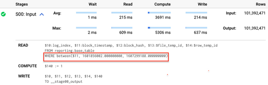
BEGINDECLARE src_range STRUCT<date_min TIMESTAMP, date_max TIMESTAMP> --115 MB processedDEFAULT(SELECT STRUCT(MIN(block_timestamp) AS date_min,MAX(block_timestamp) AS date_max) FROM staging.load_delta);MERGE INTO reporting.base_table T --41 GB processedUSING (SELECT *FROM staging.load_deltaWHERE block_timestamp BETWEEN src_range.date_min AND src_range.date_max) SON T.block_hash = S.block_hashAND T.log_index = S.log_indexAND T.block_timestamp = S.block_timestampWHEN MATCHED THEN UPDATE SETT.data = S.dataWHEN NOT MATCHED THEN INSERT (log_index, data, topics, block_timestamp, block_hash)VALUES (log_index, data, topics, block_timestamp, block_hash);END;
Note that you add the static filter to the staging table and keep T.block_timestamp = S.block_timestamp to convey to BigQuery that it can push that filter to the base table. This MERGE processes 41 GB of data in contrast to the initial 161 GB. You can see in the query plan that BigQuery pushes the partition filter from the staging table to the base table:
This type of optimization, when a pruning condition is pushed from a subquery to a large partitioned or clustered table, is not unique for MERGE. It also works for other types of queries. For instance:
SELECT * -- 41 GB processedFROM reporting.base_table TINNER JOIN staging.load_delta SON T.block_hash = S.block_hashAND T.log_index = S.log_indexAND T.block_timestamp = S.block_timestampWHERE S.block_timestamp BETWEEN TIMESTAMP '2020-10-05' AND TIMESTAMP '2020-12-07'
And you can check the query plan to verify that BigQuery pushed down the partition filter from one table to another.
Moreover, for SELECT statements, BigQuery can automatically infer a filter predicate on a join column and push it down from one table to another if your query meets the following criteria:
- The target table must be clustered or partitioned.
- The result size of the other table, i.e. after applying all filters, must qualify for broadcast join. Namly, the result set must be relatively small, less than ~100MB.
In our running example, reporting.base_table is partitioned by block_timestamp. If you define a selective filter on staging.load_delta and join two tables, you can see an inferred filter on the join key pushed to the target table
SELECT *FROM reporting.base_table TINNER JOIN staging.load_delta SON T.block_timestamp = S.block_timestampWHERE S.block_hash = '0x0c1caa16b34d94843aabfebc0d5a961db358135988f7498a6fdc450ad55f0870'
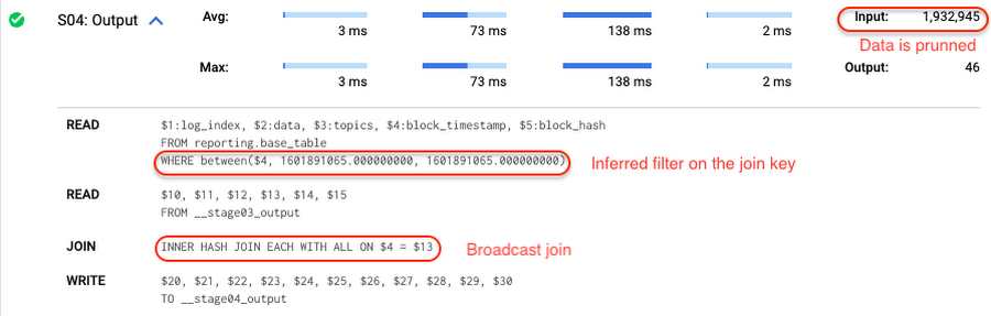
There is no requirement to join tables by partitioning or clustering key to kick off this type of optimization. However, in this case the pruning effect on the target table would be less significant.
But let us get back to the pipeline optimizations. Another way to enhance MERGE is to modify the merge_condition filter by adding static predicate on the base table:
BEGINDECLARE src_range STRUCT<date_min TIMESTAMP, date_max TIMESTAMP> --115 MB processedDEFAULT(SELECT STRUCT(MIN(block_timestamp) AS date_min,MAX(block_timestamp) AS date_max) FROM staging.load_delta);MERGE INTO reporting.base_table T --41 GB processedUSING staging.load_delta SON T.block_hash = S.block_hashAND T.log_index = S.log_indexAND T.block_timestamp BETWEEN src_range.date_min AND src_range.date_maxWHEN MATCHED THEN UPDATE SETT.data = S.dataWHEN NOT MATCHED THEN INSERT (log_index, data, topics, block_timestamp, block_hash)VALUES (log_index, data, topics, block_timestamp, block_hash);END;
To summarize, here are the steps that you can perform to enhance incremental ingestion pipelines in BigQuery. First you compute the range of updated partitions based on the small staging table. Next, you tweak the MERGE statement a bit to let BigQuery know to prune data in the base table.
All the enhanced MERGE statements scanned 41 GB of data, and setting up the src_range variable took 115 MB. Compare it with the initial 161 GB scan. Moreover, given that computing src_range may be incorporated into some existing transformation in your ETL/ELT, it results in a good performance improvement which you can leverage in your pipelines.
In this post we described how to enhance data ingestion pipelines by turning dynamic filter predicates into static predicates and letting BiQuery prune data for us. You can find more tips on BigQuery DML tuning here.
Special thanks to Daniel De Leo, who helped with examples and provided valuable feedback on this content.
Qlik and Google Cloud Combo: Extending Integration of SAP Data on BigQuery
5453
Of your peers have already read this article.
2:00 Minutes
The most insightful time you'll spend today!
If your organization is one of the 52% of SAP customers whose top analytics pain point is data integration1, Google Cloud has got you covered. By working with partners like Qlik, we are expanding our integration options and bringing real-time replication capability for SAP to BigQuery.
Integrated data for accelerated insights
BigQuery—our fully managed, enterprise data warehouse that can scale up to petabytes on demand and execute queries in seconds—allows SAP customers to consolidate enterprise data silos and confidently derive more use and value from their data. Customers can accelerate and simplify the delivery of SAP data on BigQuery with the latest Qlik Data Integration platform offering for Google Cloud which allows data integration using an automated, near real-time data pipeline through Qlik Replicate, whether data originates from legacy SAP environments, SAP HANA, or SAP application servers. Additionally, Qlik Compose for Data Warehouses can be used to easily generate and automate logical data models from SAP directly in BigQuery freeing up more time for data analysts to leverage advanced built-in capabilities such as BigQuery ML to derive greater value and insights using standard SQL without the need for advanced programming expertise.
Delivering faster results with real-time
Traditional extract-transform-load (ETL) solutions operate on a batch basis, pulling data sets from SAP daily, hourly, or every minute. These tools often require manual mapping of multiple data fields so that data flows accurately. Given SAP’s highly complex table relationships, in which a single transaction can result in multiple changes, this can be a time consuming and tedious process. ETL can also increase the burden on your SAP systems.
Qlik Replicate simplifies this with its intuitive user interface where you can set up real-time data replication between SAP and BigQuery, eliminating the need for manual coding. And, to prevent system overhead, as soon as a new transaction is entered into SAP, the resulting data is replicated into BigQuery in a process known as change data capture (CDC) from SAP’s log layer. This means that data transfer can benefit from high performance with minimal impact on the source system’s resources. Read our latest white paper to learn how to extract SAP data into BigQuery leveraging Qlik Replicate.
Solution expertise for all core SAP workloads
It doesn’t matter what database your SAP system runs on, Qlik Replicate supports all core SAP systems. It automates real-time data replication and decodes SAP’s complex, application-specific data structures into formats that flow smoothly into BigQuery. This ensures that anyone who depends on data analytics has the most current and relevant SAP data they need. For its robust solution capabilities Qlik has received a new “SAP on Google Cloud Expertise” designation for supporting:
- Fast onboarding and accelerated replication of SAP data into Google Cloud
- Real-time and continuous data replication from SAP applications to BigQuery
- Support for all core SAP modules and a broad set of data sources
- Automated data integration, which cuts resource requirements for initial delivery and ongoing maintenance
Proven customer results
Many SAP customers have experienced the benefits of leveraging Qlik alongside BigQuery for data analytics and AI at scale, including German luxury department store chain Breuninger. In order to meet its customers’ growing and changing expectations,Breuninger needed to accelerate its time to insight from data sources across a highly dispersed landscape of on-premises databases and systems, including SAP. The company uses Qlik Replicate to feed corporate data from modules in its SAP system into BigQuery and integrate its varying on-premises databases with the Google Cloud environment. This has yielded game-changing, real-time customer insights for the retailer.
What could your business do with faster, more integrated insights? Learn more about BigQuery for SAP customers and also how Qlik and Google Cloud can help you modernize and automate data integration and analytics.
More Relevant Stories for Your Company

Fortress Vault Joins Forces with Google Cloud: Launches Private Data Storage for NFTs
Over the past two years, the general population has become more acquainted with cryptocurrencies and the first iterations of NFTs, which were among the earliest use cases for blockchain technology. This public awareness and participation has led to a growing interest in, and demand for, Web3 technology at the enterprise

New to Cloud Firestore? Here are Some Basics You Need to Know
Learning to use a new database can be daunting, even more so if you don’t already have technical knowledge about databases. In this article, I will break down some database basics, terms you should know, what Firestore is, how it works, how it stores data, and how to get started
Google Leads the Pack in Big Data NoSQL Market: Forrester Research
NoSQL has become critical for all businesses to support modern business applications. It has gone from supporting simple schemaless apps to becoming a mission-critical data platform for large Fortune 1000 companies. It has already disrupted the database market, which was dominated for decades by relational database vendors. Today, half of

Daffodil Software Saves Hundreds of Hours Managing Databases with Google Cloud SQL
Daffodil Software is an India-based information technology services company with 180 employees and satellite offices in the US, Singapore, and the United Arab Emirates. Its product: A suite of web-based applications, including a business customer relationship management (CRM) program and an enterprise resource planning (ERP) app for schools. Daffodil’s Challenge
