Many of today’s games are rich, immersive worlds that engage the audience in ways that make a gamer a part of a continuing storyline. To create these persistent experiences, numerous storage technologies are required to ensure game data can scale to the standards of gamers’ demands. Not only do game developers need to store different types of data—such as saves, inventory, patches, replays, and more—but they also must keep the storage system high-performing, available, scalable, and cost-effective.

Enter Open Saves, a brand-new, purpose-built single interface for multiple storage back ends that’s powered by Google Cloud and developed in partnership with 2K. Now, development teams can store game data without having to make the technical decisions on which storage solution to use, whether that’s Cloud Storage, Memorystore, or Firestore. 

“Open Saves demonstrates our commitment to partnering with top developers on gaming solutions that require a combination of deep industry expertise and Google scale,” said Joe Garfola, Vice President of IT and Security at 2K. “We look forward to continued collaboration with Google Cloud.”

Game development teams can save game data against Open Saves without having to worry about the optimal back-end storage solution, while operations teams can focus on needed scalability and storage options. Here’s how it looks in practice:

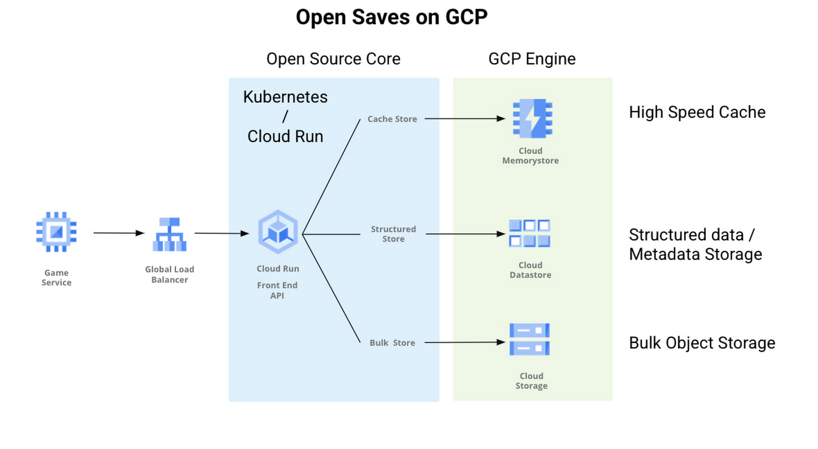
With Open Saves, game developers can run a cloud-native game storage system that is:

• Simple: Open Saves provides a unified, well-defined gRPC endpoint for all operations for metadata, structured, and unstructured objects.
• Fast: With a built-in caching system, Open Saves optimizes data placements based on access frequency and data size, all to achieve both low latency for smaller binary objects and high throughput for big objects.
• Scalable: The Open Saves API server can run on either Google Kubernetes Engine or Cloud Run. Both platforms can scale out to handle hundreds of thousands of requests per second. Open Saves also stores data in Firestore and Cloud Storage, and can handle hundreds of gigabytes of data and up to millions of requests per second.

Open Saves is designed with extensibility in mind, and can be integrated into any game—whether mobile or console, multiplayer or single player—running on any infrastructure, from on-prem to cloud or a hybrid. The server is written in Go, but you can use many programming languages and connect from client or server since the API is defined in gRPC.

Writing to and reading from Open Saves is as simple as the following code:

  // To write
	record := &pb.Record{
		Key:      uuid.New().String(),
		Tags:     []string{"tag1", "tag2"},
		OwnerId:  "owner",
	}
	createReq := &pb.CreateRecordRequest{
		StoreKey: storeKey,
		Record:   record,
	}
	_, err := client.CreateRecord(ctx, createReq)
	if err != nil {
		t.Fatalf("CreateRecord failed: %v", err)
	}
	// To read
	getReq := &pb.GetRecordRequest{StoreKey: storeKey, Key: recordKey}
	response, err := client.GetRecord(ctx, getReq)
	if err != nil {
		t.Errorf("GetRecord failed: %v", err)
	}

We are actively developing Open Saves in partnership with 2K Games, and would love for you to come join us on GitHub. There are a few ways to get involved:

• Install and deploy your Open Saves service
• Check out the API reference
• Read the development guide and start contributing
• Join the open-saves-discuss mailing list

Explainable AI (XAI) helps you understand and interpret how your machine learning models make decisions. We’re excited to announce that BigQuery Explainable AI is now generally available (GA). BigQuery is the data warehouse that supports explainable AI in a most comprehensive way w.r.t both XAI methodology and model types. It does this at BigQuery scale, enabling millions of explanations within seconds with a single SQL query.

Why is Explainable AI so important? To demystify the inner workings of machine learning models, Explainable AI is quickly becoming an essential and growing need for businesses as they continue to invest in AI and ML. With 76% of enterprises now prioritizing artificial intelligence (AI) and machine learning (ML) over other initiatives in 2021 IT budgets, the majority of CEOs (82%) believe that AI-based decisions must be explainable to be trusted according to a PwC survey.

While the focus of this blogpost is on BigQuery Explainable AI, Google Cloud provides a variety of tools and frameworks to help you interpret models outside of BigQuery, such as with Vertex Explainable AI, which includes AutoML Tables, AutoML Vision, and custom-trained models.

So how does Explainable AI in BigQuery work exactly? And how might you use it in practice? 

Two types of Explainable AI: global and local explainability

When it comes to Explainable AI, the first thing to note is that there are two main types of explainability as they relate to the features used to train the ML model: global explainability and local explainability.

Imagine that you have a ML model that predicts housing price (as a dollar amount), based on three features: (1) number of bedrooms, (2) distance to the nearest city center, and (3) construction date.

Global explainability (a.k.a. global feature importance) describes the features’ overall influence on the model and helps you understand if a feature had a greater influence than other features over the model’s predictions. For example, global explainability can reveal that the number of bedrooms and distance to city center typically has a much stronger influence than the construction date on predicting housing prices. Global explainability is especially useful if you have hundreds or thousands of features and you want to determine which features are the most important contributors to your model. You may also consider using global explainability as a way to identify and prune less important features to improve the generalizability of their models.

Local explainability (a.k.a. feature attributions) describes the breakdown of how each feature contributes towards a specific prediction. For example, if the model predicts that house ID#1001 has a predicted price of $230,000, local explainability would describe a baseline amount (e.g. $50,000) and how each of the features contributes on top of the baseline towards the predicted price. For example, the model may say that on top of the baseline of $50,000, having 3 bedrooms contributed an additional $50,000, close proximity to the city center added $100,000, and construction date of 2010 added $30,000, for a total predicted price of $230,000. In essence, understanding the exact contribution of each feature used by the model to make each prediction is the main purpose of local explainability.

What ML models does BigQuery Explainable AI apply to?

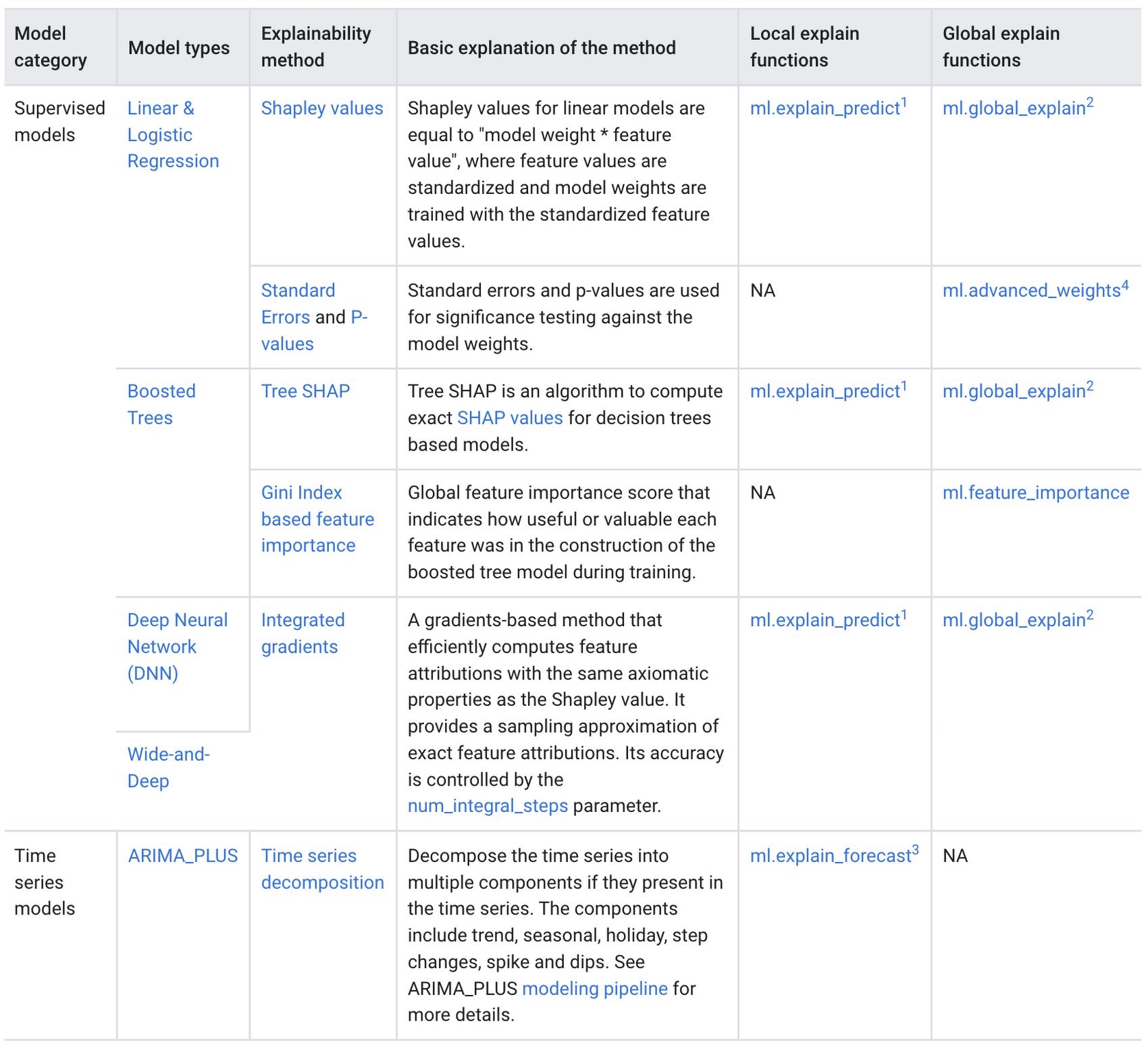
BigQuery Explainable AI applies to a variety of models, including supervised learning models for IID data and time series models. The documentation for BigQuery Explainable AI provides an overview of the different ways of applying explainability per model. Note that each explainability method has its own way of calculation (e.g. Shapley values), which are covered more in-depth in the documentation.

Examples with BigQuery Explainable AI

In this next section, we will show three examples of how to use BigQuery Explainable AI in different ML applications: 

• regression 
• classification
• time-series forecasting

Regression models with BigQuery Explainable AI

Let’s use a boosted tree regression model to predict how much a taxi cab driver will receive in tips for a taxi ride, based on features such as number of passengers, payment type, total payment and trip distance. Then let’s use BigQuery Explainable AI to help us understand how the model made the predictions in terms of global explainability (which features were most important?) and local explainability (how did the model arrive at each prediction?).

The taxi trips dataset comes from the BigQuery public datasets and is publicly available in the table: bigquery-public-data.new_york_taxi_trips.tlc_yellow_trips_2018. 

First, you can train a boosted tree regression model.

  CREATE OR REPLACE MODEL bqml_tutorial.taxi_tip_regression_model
OPTIONS (model_type='boosted_tree_regressor',
         input_label_cols=['tip_amount'],
         max_iterations = 50,
         tree_method = 'HIST',
         subsample = 0.85,
         enable_global_explain = TRUE
) AS
SELECT
  vendor_id,
  passenger_count,
  trip_distance,
  rate_code,
  payment_type,
  total_amount,
  tip_amount
FROM
  `bigquery-public-data.new_york_taxi_trips.tlc_yellow_trips_2018`
WHERE tip_amount >= 0
LIMIT 1000000

Now let’s do a prediction using ML.PREDICT, which is the standard way in BigQuery ML to make predictions without explainability.

  SELECT *
FROM
ML.PREDICT(MODEL bqml_tutorial.taxi_tip_regression_model,
 (
 SELECT
   "0" AS vendor_id,
   1 AS passenger_count,
   CAST(5.85 AS NUMERIC) AS trip_distance,
   "0" AS rate_code,
   "0" AS payment_type,
   CAST(55.56 AS NUMERIC) AS total_amount))

But you might wonder—how did the model generate this prediction of ~11.077?

BigQuery Explainable AI can help us answer this question. Instead of using ML.PREDICT, you use ML.EXPLAIN_PREDICT with an additional optional parameter top_k_features. ML.EXPLAIN_PREDICT extends the capabilities of ML.PREDICT by outputting several additional columns that explain how each feature contributes to the predicted value. In fact, since ML.EXPLAIN_PREDICT includes all the output from ML.PREDICT anyway, you may want to consider using ML.EXPLAIN_PREDICT every time instead.

  SELECT *
FROM
ML.EXPLAIN_PREDICT(MODEL bqml_tutorial.taxi_tip_regression_model,
 (
 SELECT
   "0" AS vendor_id,
   1 AS passenger_count,
   CAST(5.85 AS NUMERIC) AS trip_distance,
   "0" AS rate_code,
   "0" AS payment_type,
   CAST(55.56 AS NUMERIC) AS total_amount),
 STRUCT(6 AS top_k_features))

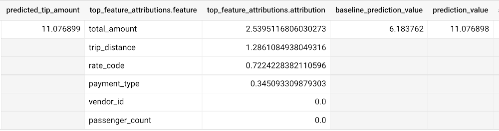
The way to interpret these columns is:

Σfeature_attributions + baseline_prediction_value = prediction_value

Let’s break this down. The prediction_value is ~11.077, which is simply the predicted_tip_amount. The baseline_prediction_value is ~6.184, which is the tip amount for an average instance. top_feature_attributions indicates how much each of the features contributes towards the prediction value. For example, total_amount contributes ~2.540 to the predicted_tip_amount. 

ML.EXPLAIN_PREDICT provides local feature explainability for regression models. For global feature importance, see the documentation for ML.GLOBAL_EXPLAIN.

Classification models with BigQuery Explainable AI

Let’s use a logistic regression model to show you an example of BigQuery Explainable AI with classification models. We can use the same public dataset as before: bigquery-public-data.new_york_taxi_trips.tlc_yellow_trips_2018.

Train a logistic regression model to predict the bracket of the percentage of the tip amount out of the taxi bill.

  CREATE OR REPLACE MODEL bqml_tutorial.taxi_tip_classification_model
OPTIONS
 (model_type='logistic_reg',
  input_label_cols=['tip_bucket'],
  enable_global_explain=true
) AS
SELECT
  vendor_id,
  passenger_count,
  trip_distance,
  rate_code,
  payment_type,
  total_amount,
  CASE
    WHEN tip_amount > total_amount*0.20 THEN '20% or more'
    WHEN tip_amount > total_amount*0.15 THEN '15% to 20%'
    WHEN tip_amount > total_amount*0.10 THEN '10% to 15%'
  ELSE '10% or less'
  END AS tip_bucket
FROM
  `bigquery-public-data.new_york_taxi_trips.tlc_yellow_trips_2018`
WHERE tip_amount >= 0
LIMIT 1000000

Next, you can run ML.EXPLAIN_PREDICT to get both the classification results and the additional information for local feature explainability. For global explainability, you can use ML.GLOBAL_EXPLAIN. Again, since ML.EXPLAIN_PREDICT includes all the output from ML.PREDICT anyway, you may want to consider using ML.EXPLAIN_PREDICT every time instead.

  SELECT *
FROM
ML.EXPLAIN_PREDICT(MODEL bqml_tutorial.taxi_tip_classification_model,
 (
 SELECT
   "0" AS vendor_id,
   1 AS passenger_count,
   CAST(5.85 AS NUMERIC) AS trip_distance,
   "0" AS rate_code,
   "0" AS payment_type,
   CAST(55.56 AS NUMERIC) AS total_amount),
 STRUCT(6 AS top_k_features))

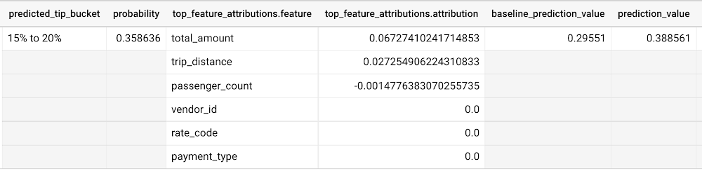
Similar to the regression example earlier, the formula is used to derive the prediction_value:

Σfeature_attributions + baseline_prediction_value = prediction_value

As you can see in the screenshot above, the baseline_prediction_value is ~0.296. total_amount is the most important feature in making this specific prediction, contributing ~0.067 to the prediction_value, though followed by trip_distance. The feature passenger_count contributes negatively to prediction_value by -0.0015. The features vendor_id, rate_code, and payment_type did not seem to contribute much to the prediction_value.

You may wonder why the prediction_value of ~0.389 doesn’t equal the probability value of  ~0.359. The reason is that unlike for regression models, for classification models, prediction_value is not a probability score. Instead, prediction_value is the logit value (i.e., log-odds) for the predicted class, which you could separately convert to probabilities by applying the softmax transformation to the logit values. For example, a three-class classification has a log-odds output of [2.446, -2.021, -2.190]. After applying the softmax transformation, the probability of these class predictions is [0.9905, 0.0056, 0.0038].

Time-series forecasting models with BigQuery Explainable AI

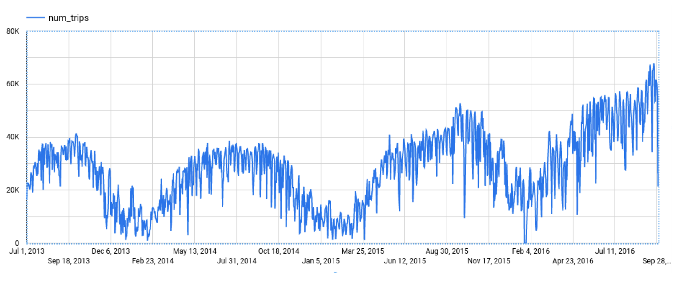
Explainable AI for forecasting provides more interpretability into how the forecasting model came to its predictions. Let’s go through an example of forecasting the number of bike trips in NYC using the new_york.citibike_trips public data in BigQuery.

You can train a time-series model ARIMA_PLUS:

  CREATE OR REPLACE MODEL bqml_tutorial.nyc_citibike_arima_model
OPTIONS
  (model_type = 'ARIMA_PLUS',
   time_series_timestamp_col = 'date',
   time_series_data_col = 'num_trips',
   holiday_region = 'US'
  ) AS
SELECT
   EXTRACT(DATE from starttime) AS date,
   COUNT(*) AS num_trips
FROM
  `bigquery-public-data.new_york.citibike_trips`
GROUP BY date

Next, you can first try forecasting without explainability using ML.FORECAST:
SELECT
  *
FROM
  ML.FORECAST(MODEL bqml_tutorial.nyc_citibike_arima_model,
              STRUCT(365 AS horizon, 0.9 AS confidence_level))

This function outputs the forecasted values and the prediction interval. Plotting it in addition to the input time series gives the following figure.

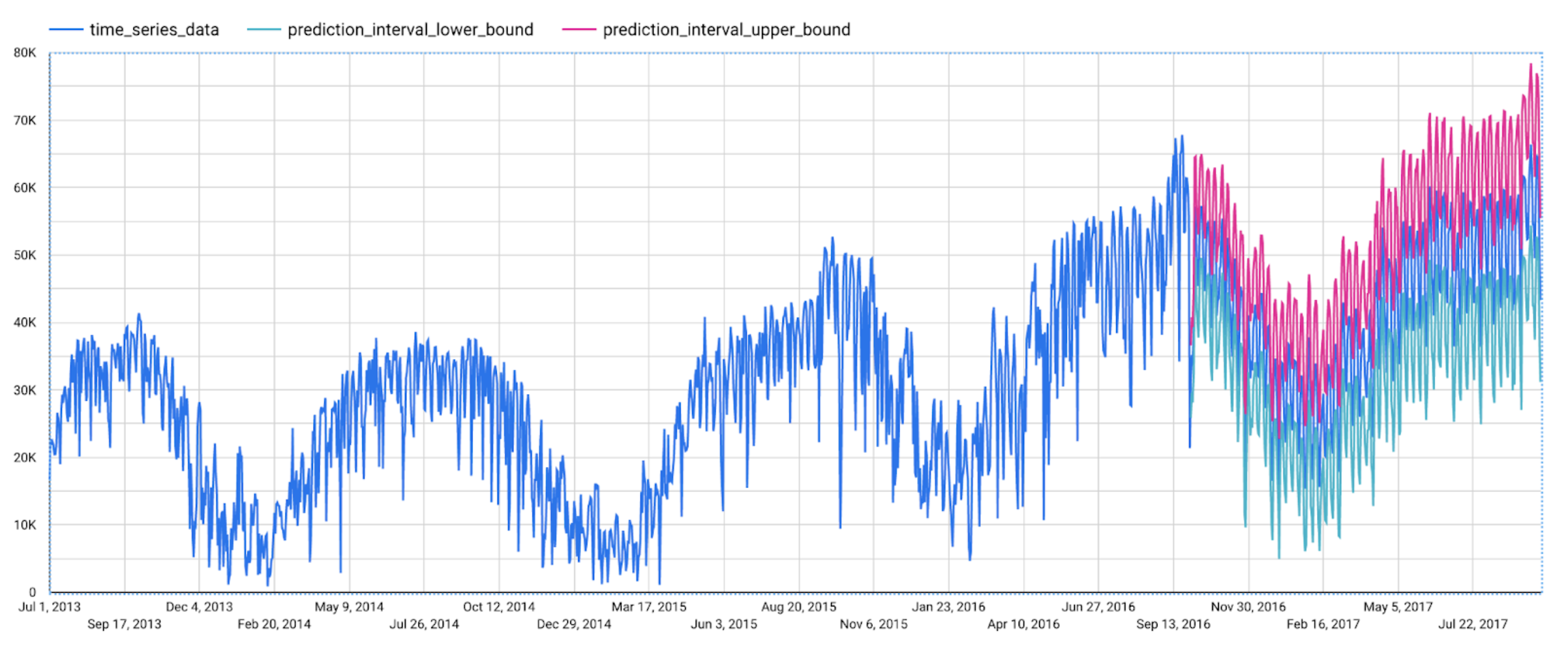
But how does the forecasting model arrive at its predictions? Explainability is especially important if the model ever generates unexpected results.

With ML.EXPLAIN_FORECAST, BigQuery Explainable AI provides extra transparency into the seasonality, trend, holiday effects, level (step) changes, and spikes and dips outlier removal. In fact, since ML.EXPLAIN_FORECAST includes all the output from ML.FORECAST anyway, you may want to consider using ML.EXPLAIN_FORECAST every time instead.

  SELECT
  *
FROM
  ML.EXPLAIN_FORECAST(MODEL bqml_tutorial.nyc_citibike_arima_model,
                      STRUCT(365 AS horizon, 0.9 AS confidence_level))

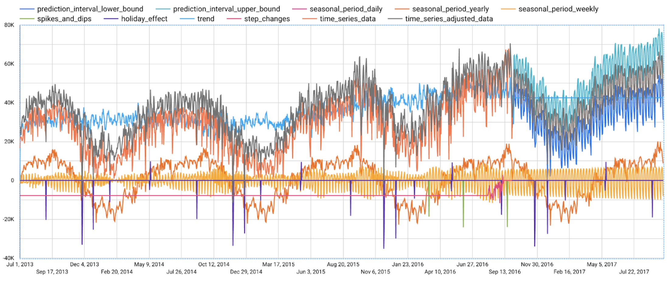
Compared to the previous figure which only shows the forecasting results, this figure shows much richer information to explain how the forecast is made.  

First, it shows how the input time series is adjusted by removing the spikes and dips anomalies, and by compensating the level changes. That is:

time_series_adjusted_data = time_series_data - spikes_and_dips - step_changes

Second, it shows how the adjusted input time series is decomposed into different components such as both weekly and yearly seasonal components, holiday effect component and trend component. That is

time_series_adjusted_data = trend + seasonal_period_yearly + seasonal_period_weekly + holiday_effect + residual

Finally, it shows how these components are forecasted separately to compose the final forecasting results. That is:

time_series_data = trend + seasonal_period_yearly + seasonal_period_weekly + holiday_effect

For more information on these time series components, please see the documentation here.

Conclusion

With the GA of BigQuery Explainable AI, we hope you will now be able to interpret your machine learning models with ease. 

Thanks to the BigQuery ML team, especially Lisa Yin, Jiashang Liu, Amir Hormati, Mingge Deng, Jerry Ye and Abhinav Khushraj. Also thanks to the Vertex Explainable AI team, especially David Pitman and Besim Avci.

Customers love Cloud Spanner because it gives them the benefits of relational semantics and SQL while also delivering the scale and availability of non-relational databases. Many of these customers want to move even more of their work to Spanner, and have requested smaller instance sizes to support development, testing and small production workloads. We’re happy to announce that they’ll soon get what they asked for: more granular instance sizing is coming to Spanner.

Granular instance sizing will be available in Public Preview soon. With this feature, you can run workloads on Spanner at as low as 1/10th the cost of regular instances, equating to approximately $65/month.

In addition, we are launching new enterprise capabilities to break down operational silos for real-time insights and provide greater database observability to developers: 

• Datastream, now in public preview, is a change data capture (CDC) service that allows enterprises to synchronize data across heterogeneous databases and applications. With Spanner support in Datastream, users will be able to stream data from MySQL or Oracle to Spanner reliably and with minimal latency. 
• BigQuery federation to Spanner (coming soon) lets users query transactional data residing in Spanner, from BigQuery, without moving or copying data. 
• Key Visualizer, available now in public preview, provides interactive monitoring so developers can quickly identify trends and usage patterns in Spanner. 

Democratizing access with more granular instance sizing 

Today, customers provision Spanner instances by specifying the number of nodes they need to run their workloads. Each node can provide up to 10,000 queries per second (QPS) of reads or 2,000 QPS of writes (writing single rows at 1 KB of data per row) and 2 TB of storage. A Spanner node is replicated across 3 zones for regional instances, and 5 or more zones for multi-regional instances. The choice of node count determines the amount of serving and storage resources that are available to the databases in a given instance. 

Historically, the most granular unit for provisioning resources on Spanner has been one node. To enable more granular control, we are introducing Processing Units (PUs); one Spanner node is equal to 1,000 PUs. Customers can now provision in batches of 100 PUs, and get a proportionate amount of compute and storage resources. This will allow teams to run smaller workloads on Spanner at much lower cost. With this feature, customers can start at 100 PUs and scale up as needed in batches of 100 PUs, to up to 1,000 PUs (1 node), all with zero downtime. Subsequently, customers can continue to scale up by adding more nodes, just like what they do today. Customers do have the choice of using either PUs or nodes to provision resources within workloads, when those workloads occupy multiple nodes of capacity. 

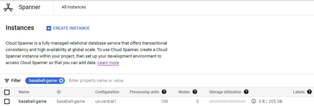
To illustrate with an example, let’s say a game developer creates a Spanner instance called “baseball-game” in us-central1, with 100 PU compute capacity at $65/month price.

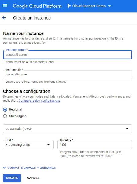
As you can see below, proportional maximum storage of 205 GB is assigned to the 100 PU instance.

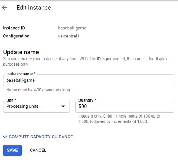
Once the game starts becoming popular and resource demands increase, the user edits the instance to increase the compute capacity to 500 PUs with proportional maximum 1 TB of storage.

The game grows in popularity, and the gaming company prepares to launch a much-awaited capability in the game. Anticipating a sharp increase in usage at launch day, the game developers increase the compute capacity to 3,000 PUs. Compute capacity assigned to the instance over a period of time can be viewed in Cloud Monitoring graphs:

Request Access 
You can request early access to granular instance sizing feature by filling this form.

Breaking down operational silos with Datastream CDC and BigQuery federation

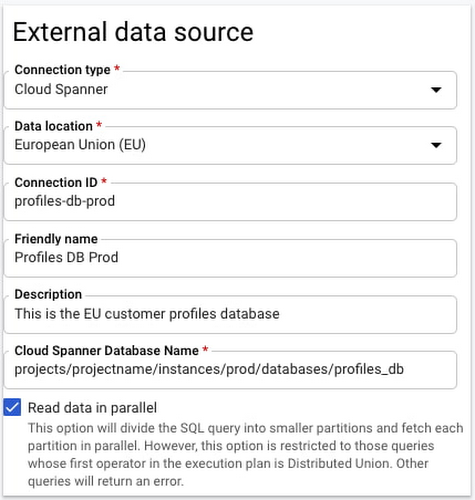
BigQuery Federation. BigQuery has made analytics easy by bringing together data from multiple sources for seamless analysis. Soon you’ll also be able to analyze data in Spanner directly in BigQuery. With  Spanner’s BigQuery federation, you’ll be able to instantly query data residing in Spanner in real-time without moving or copying the data. Simply set up the Spanner as an external data source in BigQuery, as shown below.

Change Data Capture ingest. Now in public preview, Datastream lets you stream change data into Google Cloud from MySQL and Oracle databases. As of today, you can ingest this change data directly into Spanner using a built-in Dataflow template. This lets you migrate data from MySQL and Oracle databases into Spanner in near-real time.

Understanding performance and resource usage with Key Visualizer

Key Visualizer is a new interactive monitoring tool that lets developers and administrators analyze usage patterns in Spanner. It reveals trends and outliers in key performance and resource metrics for databases of any size, helping to optimize queries and reduce infrastructure costs. Designed for performance tuning and instance sizing, Key Visualizer is available today in public preview in the web-based Cloud Console for all Spanner databases at no additional cost. Learn more in the Key Visualizer blog. 

Learn more

• To request early access to granular instance sizing in Spanner, fill out this form.
• To get started with Spanner today, create an instance or try it out with a Spanner Qwiklab.