





Over 700 SaaS Companies Trust Google’s Data Cloud to Build Intelligent Apps!

3497
Of your peers have already read this article.
5:00 Minutes
The most insightful time you'll spend today!
Today, a typical enterprise uses over 100 SaaS applications while large organizations commonly use over 400 apps. These applications contain valuable data on customers, suppliers, employees, products and more, offering the potential for valuable insights and powerful workflows. However, in the past, this data has often remained siloed and underutilized, even within an application.
Customer demand is driving an unprecedented wave of innovation across the SaaS industry, with providers building intelligence into their applications through rich analytical and AI/ML capabilities, and enabling their customers’ data ecosystems through real time data sharing. The data cloud platform powering these applications is a critical factor in companies’ ability to innovate and optimize efficiency, while keeping its customer’s data secure.
Today, over 700 tech companies including Zoominfo, Equifax, Exabeam, Bloomreach, and Quantum Metric power their products and businesses using Google’s data cloud. This week at the Data Cloud Summit, we announced the Built with BigQuery initiative which helps ISVs get started building applications using data and machine learning products. By providing dedicated access to technology, expertise and go to market programs, this initiative allows tech companies to accelerate, optimize and amplify their success.
“Enabling customers to gain superior insights and intelligence from data is core to the ZoomInfo strategy,” ZoomInfo CEO Henry Schuck says. “We are excited about the innovation Google Cloud is bringing to market and how it is creating a differentiated ecosystem that allows customers to gain insights from their data securely, at scale, and without having to move data around. Working with the Built with BigQuery initiative team enables us to rapidly gain deep insight into the opportunities available and accelerate our speed to market.”
Building intelligent SaaS applications with a unified data platform
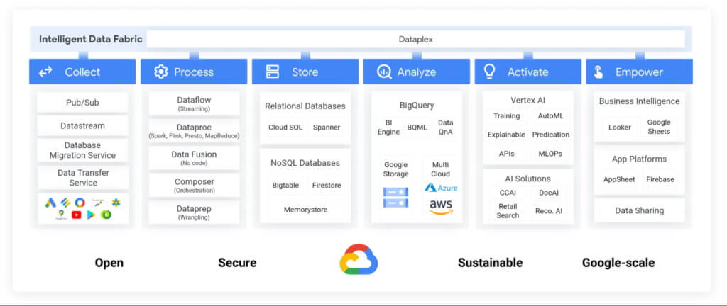
Google’s data cloud provides a complete platform for building data-driven applications, from simplified data ingestion, processing and storage to powerful analytics, AI/ML and data sharing capabilities, all seamlessly integrated with Google Cloud’s open, secure, sustainable platform. With a huge partner ecosystem and support for multicloud, open source tools and APIs, we provide technology companies the portability and extensibility they need to avoid data lock-in.
Through the Built with BigQuery initiative, we are helping tech companies to build the next-gen SaaS applications on Google’s data cloud with simplified access to technology, dedicated engineering support and joint go to market programs.
Exabeam, a next generation cybersecurity solution, is a great example. The company leverages Google’s data cloud to provide their customers with a “limitless-scale” cybersecurity solution.
“Built with Google’s data cloud, Exabeam’s limitless-scale cybersecurity platform helps enterprises respond to security threats faster and more accurately” said Sanjay Chaudhary, VP of Products at Exabeam. “We are able to ingest data from over 500 security vendors, convert unstructured data into security events, and create a common platform to store them in a cost effective way. The scale and power of Google’s data cloud enables our customers to search multi-year data and detect threats in seconds.”
Foster innovation and unlock new business models through data sharing
Data becomes even more valuable when shared. According to research, the global data monetization market size is growing at a CAGR of 47.9% and is projected to reach $11.7 Billion by 2026. It’s a compelling proposition for SaaS companies as it enables them to deliver increased value for their customers while expanding their own partner ecosystem, increasing stickiness and unlocking new revenue streams.
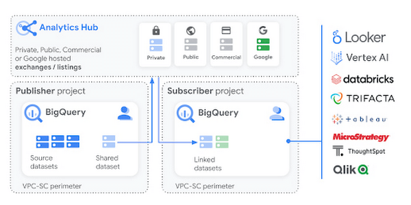
Google Cloud’s strategy for data sharing encompasses three key areas: secure data sharing in BigQuery, the ability to create private and public exchanges alongside commercial and public datasets in Analytics Hub, and a robust ecosystem of premier partner and Google data.
Through the real-time data sharing capabilities of BigQuery, SaaS companies are enabling their customers to combine their data with the customer’s own proprietary data, and other third-party data sources, to derive 360-degree insights. Over 4,500 organizations share more than 250 Petabytes of data weekly in BigQuery, not accounting for intra-organizational data sharing*.
For example, manufacturers can get real-time visibility into their entire supply chain by combining datasets from ISVs, such as supply chain innovator, Blume Global, and data publishers.
“Our partnership with Google Cloud is helping us achieve our mission to build the next-generation supply chain operating system. Blume Maps, our digital twin of the supply chain world built with Google’s data cloud, allows our customers to generate accurate lead times, real-time shipment location and ETAs” said Blume Global CEO Pervinder Johar. “We apply the power of Google Cloud’s data and analytics capabilities to our growing database of over 1.5 million global data points to feed our lead time and dynamic ETA engine. We are also able to create data twins of unique logistics data and share with users around the globe.”
Google Cloud’s Analytics Hub is a fully-managed service built on BigQuery that allows organizations to efficiently and securely exchange valuable data and analytics assets across any organizational boundary. With unique datasets that are always-synchronized and bi-directional sharing, you can create a rich and trusted data ecosystem between business units or partnerships–one in which everyone gains value immediately.
“As external data becomes more critical to organizations across industries, the need for a unified experience between data integration and analytics has never been more important. We are proud to be working with Google Cloud to power the launch of Analytics Hub, feeding hundreds of pre-engineered data pipelines from hundreds of external datasets,” said Dan Lynn, SVP Product at Crux. “The sharing capabilities that Analytics Hub delivers will significantly enhance the data mobility requirements of practitioners, and the Crux data integration platform stands ready to quickly integrate any external data source and deliver on behalf of Google Cloud and its clients.”
Innovate, optimize and amplify with Google Cloud
The Built with BigQuery initiative provides access to technology, expertise and go-to-market:.
- Access to Technology: Get started fast with a Google-funded, pre-configured sandbox. Access Cloud Credits to fund your, and your customer’s, POCs and apply for innovative pricing models designed for ISVs.
- Access to Expertise: Accelerate and optimize product design and architecture with access to designated experts in building data-driven SaaS applications from the ISV Center of Excellence, providing insight into key use cases, architectural patterns and best practices. Access experts from across Google to enable co-innovation with products such as Earth Engine and Google Marketing Platform.
- Access to Go-to-market: Amplify your success with joint marketing programs to drive awareness, generate demand and increase adoption.
Get Started
Start building your applications on Google Cloud with $300 in free credits or apply for the Built with BigQuery initiative.
*As of November, 2021, within a typical 7 day period in BigQuery, and not accounting for intra-organizational data sharing.
What’s Google Cloud Firestore Database and What are it’s Benefits for Business and Developers?
5983
Of your peers have already read this article.
2:30 Minutes
The most insightful time you'll spend today!
Cloud Firestore is a NoSQL document database that simplifies storing, syncing, and querying data for your mobile and web apps at global scale.
Cloud Firestore is a fast, fully managed, serverless, cloud-native NoSQL document database that simplifies storing, syncing, and querying data for your mobile, web, and IoT apps at global scale.
Its client libraries provide live synchronization and offline support, while its security features and integrations with Firebase and Google Cloud Platform (GCP) accelerate building truly serverless apps.
Here’s other stuff it’s good at:
Sync data across devices, on or offline
With Cloud Firestore, your applications can be updated in near real time when data on the back end changes. This is not only great for building collaborative multi-user mobile applications, but also means you can keep your data in sync with individual users who might want to use your app from multiple devices.
With Firebase Realtime Database, we felt we had built the best force-plate testing software on the market. Thanks to Cloud Firestore, in only two weeks, we built a system that’s significantly better and includes features we never thought possible to ship on Day 1.
Chris Wales, CTO, Hawkin Dynamics
Cloud Firestore has full offline support, so you can access and make changes to your data, and those changes will be synced to the cloud when the client comes back online. Built-in offline support leverages local cache to serve and store data, so your app remains responsive regardless of network latency or internet connectivity.
Simple and effortless
Cloud Firestore’s robust client libraries make it easy for you to update and receive new data while worrying less about establishing network connections or unforeseen race conditions. It can scale effortlessly as your app grows. Cloud Firestore allows you to run sophisticated queries against your data. This gives you more flexibility in the way you structure your data and can often mean that you have to do less filtering on the client, which keeps your network calls and data usage more efficient.
Enterprise-grade, scalable NoSQL
Cloud Firestore is a fast and fully managed NoSQL cloud database. It is built to scale and takes advantage of GCP’s powerful infrastructure, with automatic horizontal scaling in and out, in response to your application’s load. Security access controls for data are built in and enable you to handle data validation via a configuration language.
Case Study: When Database Choice Powers New Revenue-driving Product Features

4173
Of your peers have already read this article.
4:30 Minutes
The most insightful time you'll spend today!
Editor’s note: Streak makes a CRM add-on for Gmail, and recently adopted Cloud Spanner to take advantage of its scalability and SQL capabilities to implement a graph data model. Read on to learn about their decision, what they love about the system, and the ways in which it still needs work.]
Streak is a customer relationship management (CRM) tool built directly into Gmail. It is used for sales, marketing, hiring, and just about anything else you can think of.
We built it because out of the box, email is actually a really crummy team sharing system. By adding a layer of organization on top of email, Streak lets you add email threads directly into its spreadsheet view, making it useful as a workflow tool with capabilities including task creation, email template management, and easy data entry.
Streak has been integrated with G Suite (originally Google Apps For Your Domain) since its inception so when choosing a cloud, it made sense to colocate our server stack with Google Cloud.
Likewise, Streak was on Google App Engine from the start, and we slowly added other GCP services as the offerings improved or as our use cases became more complex.
In addition to App Engine, we use Google Kubernetes Engine to run a bunch of our compute workload, including both application servers and our offline processes like indexers and task queue consumers.
We use Cloud Dataflow for both streaming event processing and logs ETL, and BigQuery for all of our analytics queries. We use Cloud Pub/Sub for interacting with the Gmail watch API, as well as Stackdriver (logging, tracing, monitoring, errors) and OpenCensus to dig into any operational issues as they arise.
Then, on the database front, we recently started using Cloud Spanner, Google Cloud’s scalable relational database service. Before that, we stored most of our business data in Cloud Datastore, Google Cloud’s NoSQL document database.
Partially, that was historical, since Cloud Datastore was GCP’s only managed database when we wrote the Streak backend. And we’ve been very happy with how easy Cloud Datastore is to maintain. Between Google App Engine and Cloud Datastore, we’ve never had to have an explicit infrastructure on-call rotation.
But as more users rely on Streak to collaborate with larger and larger teams, we were feeling the pain of not having a fully relational database. We found ourselves having to manually join data in our application, which increased application latency and increased the time developers spent coding workarounds and debugging that complexity.
We found we needed two things out of our database: a scalable relational store and a graph store that could power next-gen Streak features. At the same time, we wanted a single database that could handle both use cases and wouldn’t increase our operational burden. This meant finding a managed service to give us more query flexibility, so we decided to give Cloud Spanner a try.
Of course, we didn’t want to migrate our existing stack to a new data platform without first testing it out (never a smart strategy). But since most of our existing data model required transactional updates with other entities, pulling out a single entity to test was challenging. We did have a feature in our pipeline that necessitated a graph data store and that was removed from our other data: our email metadata indexing system.
How your client software handles email metadata indexing can make or break the useability of a system. Think about how many times somebody forgets to reply-all or that you receive a forwarded thread with thirty emails in reverse-chronological order. Within our own inboxes, we rely on Gmail’s UI to nicely organize email threads, but that organization breaks down when working with a team or across organizational boundaries.
We decided to fix that in the Streak product by organizing metadata (i.e., headers but not message content) from users’ email by using Cloud Spanner as a graph database. Using a graph database lets us answer questions like “What are all the emails on this thread in the inboxes of everybody on my team?” and “Who on my team has previously talked with the organization that this prospect works at?”
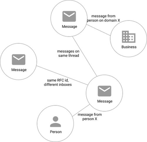
In our model, the nodes of the graph are either an email message, a person (email address) or a company (a domain). Then we have four different types of “edges”— properties by which nodes in a graph connect to one another:
- Message to message (thread): messages that are on the same thread have an edge between them. The reason we do this is because we want to show users a list of threads to answer their questions, not messages, so we need to be able to get the spanning set of messages.
- Message to message (same RFC id): A core value proposition of Streak is being able to see the “unified” version of a thread that shows each person on a team’s version of the email thread. To make sure we are getting each user’s version of a thread when we issue a query, there needs to be an edge between a message in the queryer’s inbox and the same message in their team’s inbox. In case you’re curious, Streak uses the RFC message id to determine that two messages across inboxes are actually the same.
- Email address to message: a message has an edge to an email address if it was either the from, to, cc, or bcc on the message. This edge is crucial for queries that start with: “Show me all threads between this person and our team.”
Domain to message: a message has an edge to a domain if the domain is present in any of the from, to, cc, or bcc addresses on the message. This edge is similarly used for queries that start with “Show me all threads between this company and our team.”
Using Cloud Spanner’s distributed SQL capabilities and scalability to build a graph database also let us answer the important follow-up question: “Which threads have I been granted permission to view?” And while a lot of these questions could be answered per-user by a traditional relational database, scale limitations have to be taken into consideration, especially as we plan for 10x or more data volume growth as both our user base grows and as their inboxes accumulate more emails. A graph database model is simply a better fit for Streak’s collaboration model with many-to-many mappings between users and teams, and will allow us to query the data in any number of configurations, without worrying about scale limitations or having to manually shard a relational database. Cloud Spanner gives us queryability and scalability.
Taking the Cloud Spanner plunge
With so many advantages to it, we went ahead and began building out our metadata system with Cloud Spanner as a back-end.
Adopting Cloud Spanner has been great. Here are some of the high points:
- The fast distributed queries and transactions are absolutely real. We have global indexes across our entire dataset and we haven’t had to spend very much time at all thinking about co-locating data. In particular, we only use interleaved tables for values that would be repeated fields in Cloud Datastore, and that hasn’t been a problem for us yet.
- We haven’t had any reliability problems whatsoever, despite averaging 20K writes/sec in steady state.
- Once we optimized our queries on realistic data, Cloud Spanner scaled up in a surprisingly predictable way. You need to run queries after you’ve populated data, do the explain to figure out how the query planner is executing the query, and add indexes/modify queries to make sure they’re performant.
- Compared to the hoops some traditional relational databases make you jump through, Cloud Spanner’s online schema changes and index builds are magical. There is no downtime for these operations.
Overall, the experience has been encouraging, and we’re planning to move 20 TB of existing data in Cloud Datastore to Cloud Spanner as well. We built out an ORM library for Java on top of Cloud Spanner called Ratchet and are testing a framework for dual-writing entities to both Cloud Datastore and Cloud Spanner to support the rest of the migration. We now store about 40 TB of email metadata in Cloud Spanner, which makes us a large user of Cloud Spanner.
In short, if you’re starting to outgrow your NoSQL database, and want to move to a managed SQL database, give Cloud Spanner a try. You definitely want to model out your costs and try out a proof of concept, both to see how it works on your workload and to get familiar with the quirks of the system. But you don’t need to spend much time worrying about the reliability of the product: it’s there.
10191
Of your peers have already watched this video.
1:00 Minutes
The most insightful time you'll spend today!
Predict User Churn on Gaming Apps with Google Analytics Data using BigQuery ML
User retention can be a major challenge for mobile game developers. According to the Mobile Gaming Industry Analysis in 2019, most mobile games only see a 25% retention rate for users after the first day. To retain a larger percentage of users after their first use of an app, developers can take steps to motivate and incentivize certain users to return. But to do so, developers need to identify the propensity of any specific user returning after the first 24 hours.
In this blog post, we will discuss how you can use BigQuery ML to run propensity models on Google Analytics 4 data from your gaming app to determine the likelihood of specific users returning to your app.
You can also use the same end-to-end solution approach in other types of apps using Google Analytics for Firebase as well as apps and websites using Google Analytics 4. To try out the steps in this blogpost or to implement the solution for your own data, you can use this Jupyter Notebook.
Using this blog post and the accompanying Jupyter Notebook, you’ll learn how to:
- Explore the BigQuery export dataset for Google Analytics 4
- Prepare the training data using demographic and behavioural attributes
- Train propensity models using BigQuery ML
- Evaluate BigQuery ML models
- Make predictions using the BigQuery ML models
- Implement model insights in practical implementations
Google Analytics 4 (GA4) properties unify app and website measurement on a single platform and are now default in Google Analytics. Any business that wants to measure their website, app, or both, can use GA4 for a more complete view of how customers engage with their business. With the launch of Google Analytics 4, BigQuery export of Google Analytics data is now available to all users. If you are already using a Google Analytics 4 property, you can follow this guide to set up exporting your GA data to BigQuery.
Once you have set up the BigQuery export, you can explore the data in BigQuery. Google Analytics 4 uses an event-based measurement model. Each row in the data is an event with additional parameters and properties. The Schema for BigQuery Export can help you to understand the structure of the data.
In this blogpost, we use the public sample export data from an actual mobile game app called “Flood It!” (Android, iOS) to build a churn prediction model. But you can use data from your own app or website.
Here’s what the data looks like. Each row in the dataset is a unique event, which can contain nested fields for event parameters.
SELECT *FROM `firebase-public-project.analytics_153293282.events_*`TABLESAMPLE SYSTEM (1 PERCENT)
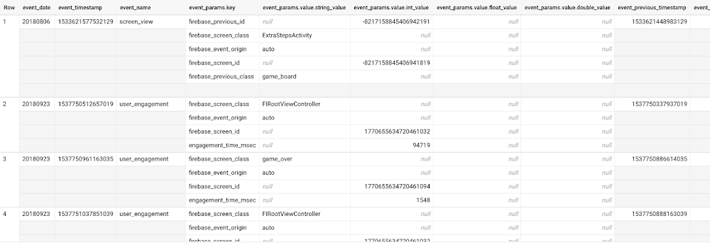
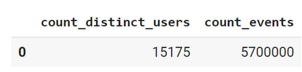
This dataset contains 5.7M events from over 15k users.
SELECTCOUNT(DISTINCT user_pseudo_id) as count_distinct_users,COUNT(event_timestamp) as count_eventsFROM`firebase-public-project.analytics_153293282.events_*
Our goal is to use BigQuery ML on the sample app dataset to predict propensity to user churn or not churn based on users’ demographics and activities within the first 24 hours of app installation.
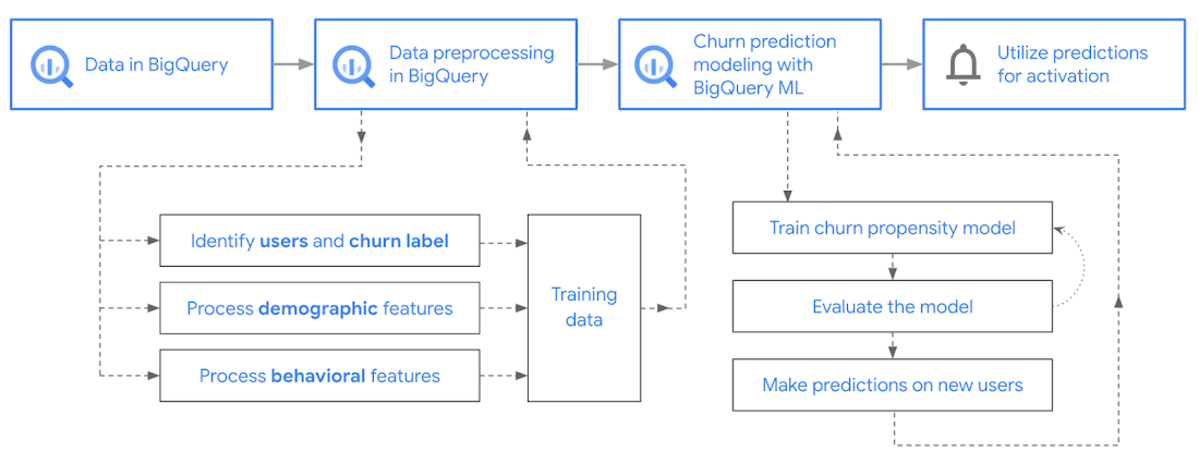
In the following sections, we’ll cover how to:
- Pre-process the raw event data from GA4
- Identify users & the label feature
- Process demographic features
- Process behavioral features
- Train classification model using BigQuery ML
- Evaluate the model using BigQueryML
- Make predictions using BigQuery ML
- Utilize predictions for activation
Pre-process the raw event data
You cannot simply use raw event data to train a machine learning model as it would not be in the right shape and format to use as training data. So in this section, we’ll go through how to pre-process the raw data into an appropriate format to use as training data for classification models.
This is what the training data should look like for our use case at the end of this section:
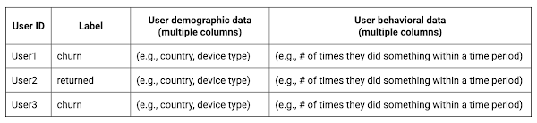
Notice that in this training data, each row represents a unique user with a distinct user ID (user_pseudo_id).
Identify users & the label feature
We first filtered the dataset to remove users who were unlikely to return the app anyway. We defined these ‘bounced’ users as ones who spent less than 10 mins with the app. Then we labeled all remaining users:
- churned: No event data for the user after 24 hours of first engaging with the app.
- returned: The user has at least one event record after 24 hours of first engaging with the app.
For your use case, you can have a different definition of bounce and churning. Also you can even try to predict something else other than churning, e.g.:
- whether a user is likely to spend money on in-game currency
- likelihood of completing n-number of game levels
- likelihood of spending n amount of time in-game etc.
In such cases, label each record accordingly so that whatever you are trying to predict can be identified from the label column.
From our dataset, we found that ~41% users (5,557) bounced. However, from the remaining users (8,031), ~23% (1,883) churned after 24 hours:
SELECTbounced,churned,COUNT(churned) as count_usersFROMbqmlga4.returningusersGROUP BY 1,2ORDER BY bounced
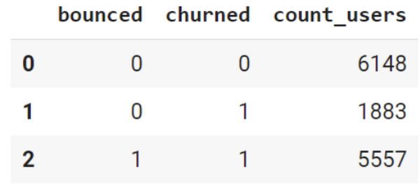
To create these bounced and churned columns, we used the following snippet of SQL code.
...#churned = 1 if last_touch within 24 hr of app installation, else 0IF (user_last_engagement < TIMESTAMP_ADD(user_first_engagement,INTERVAL 24 HOUR),1,0 ) AS churned,#bounced = 1 if last_touch within 10 min, else 0IF (user_last_engagement <= TIMESTAMP_ADD(user_first_engagement,INTERVAL 10 MINUTE),1,0 ) AS bounced,...
You can view the Jupyter Notebook for the full query used for materializing the bounced and churned labels.
Process demographic features
Next, we added features both for demographic data and for behavioral data spanning across multiple columns. Having a combination of both demographic data and behavioral data helps to create a more predictive model.
We used the following fields for each user as demographic features:
geo.countrydevice.operating_systemdevice.language
A user might have multiple unique values in these fields — for example if a user uses the app from two different devices. To simplify, we used the values from the very first user engagement event.
CREATE OR REPLACE VIEW bqmlga4.user_demographics AS (WITH first_values AS (SELECTuser_pseudo_id,geo.country as country,device.operating_system as operating_system,device.language as language,ROW_NUMBER() OVER (PARTITION BY user_pseudo_id ORDER BY event_timestamp DESC) AS row_numFROM `firebase-public-project.analytics_153293282.events_*`WHERE event_name="user_engagement")SELECT * EXCEPT (row_num)FROM first_valuesWHERE row_num = 1 #first engagement);
Process behavioral features
There is additional demographic information present in the GA4 export dataset, e.g. app_info, device, event_params, geo etc. You may also send demographic information to Google Analytics through each hit via user_properties. Furthermore, if you have first-party data on your own system, you can join that with the GA4 export data based on user_ids.
To extract user behavior from the data, we looked into the user’s activities within the first 24 hours of first user engagement. In addition to the events automatically collected by Google Analytics, there are also the recommended events for games that can be explored to analyze user behavior. For our use case, to predict user churn, we counted the number of times the follow events were collected for a user within 24 hours of first user engagement:
user_engagementlevel_start_quickplaylevel_end_quickplaylevel_complete_quickplaylevel_reset_quickplaypost_scorespend_virtual_currencyad_rewardchallenge_a_friendcompleted_5_levelsuse_extra_steps
The following query shows how these features were calculated:
WITHevents_first24hr AS (SELECTe.*FROM`firebase-public-project.analytics_153293282.events_*` eJOINbqmlga4.returningusers rONe.user_pseudo_id = r.user_pseudo_idWHERETIMESTAMP_MICROS(e.event_timestamp) <= r.ts_24hr_after_first_engagement)SELECTuser_pseudo_id,SUM(IF(event_name = 'user_engagement', 1, 0)) AS cnt_user_engagement,# ... repeated for all behavior data ...SUM(IF(event_name = 'use_extra_steps', 1, 0)) AS cnt_use_extra_steps,FROMevents_first24hrGROUP BY1
View the notebook for the query used to aggregate and extract the behavioral data. You can use different sets of events for your use case. To view the complete list of events, use the following query:
SELECTevent_name,COUNT(event_name) as event_countFROM`firebase-public-project.analytics_153293282.events_*`GROUP BY 1ORDER BYevent_count DESC
After this we combined the features to ensure our training dataset reflects the intended structure. We had the following columns in our table:
- User ID:
user_pseudo_id
- Label:
churned
- Demographic features
countrydevice_osdevice_language
- Behavioral features
cnt_user_engagementcnt_level_start_quickplaycnt_level_end_quickplaycnt_level_complete_quickplaycnt_level_reset_quickplaycnt_post_scorecnt_spend_virtual_currencycnt_ad_rewardcnt_challenge_a_friendcnt_completed_5_levelscnt_use_extra_stepsuser_first_engagement
At this point, the dataset was ready to train the classification machine learning model in BigQuery ML. Once trained, the model will output a propensity score between churn (churned=1) or return (churned=0) indicating the probability of a user churning based on the training data.
Train classification model
When using the CREATE MODEL statement, BigQuery ML automatically splits the data between training and test. Thus the model can be evaluated immediately after training (see the documentation for more information).
For the ML model, we can choose among the following classification algorithms where each type has its own pros and cons:
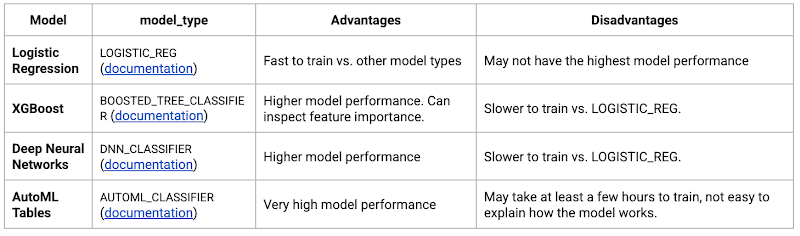
Often logistic regression is used as a starting point because it is the fastest to train. The query below shows how we trained the logistic regression classification models in BigQuery ML.
CREATE OR REPLACE MODEL bqmlga4.churn_logregTRANSFORM(EXTRACT(MONTH from user_first_engagement) as month,EXTRACT(DAYOFYEAR from user_first_engagement) as julianday,EXTRACT(DAYOFWEEK from user_first_engagement) as dayofweek,EXTRACT(HOUR from user_first_engagement) as hour,* EXCEPT(user_first_engagement, user_pseudo_id))OPTIONS(MODEL_TYPE="LOGISTIC_REG",INPUT_LABEL_COLS=["churned"]) ASSELECT*FROMbqmlga4.train
We extracted month, julianday, and dayofweek from datetimes/timestamps as one simple example of additional feature preprocessing before training. Using TRANSFORM() in your CREATE MODEL query allows the model to remember the extracted values. Thus, when making predictions using the model later on, these values won’t have to be extracted again. View the notebook for the example queries to train other types of models (XGBoost, deep neural network, AutoML Tables).
Evaluate model
Once the model finished training, we ran ML.EVALUATE to generate precision, recall, accuracy and f1_score for the model:
SELECT*FROMML.EVALUATE(MODEL bqmlga4.churn_logreg)

The optional THRESHOLD parameter can be used to modify the default classification threshold of 0.5. For more information on these metrics, you can read through the definitions on precision and recall, accuracy, f1-score, log_loss and roc_auc. Comparing the resulting evaluation metrics can help to decide among multiple models.Furthermore, we used a confusion matrix to inspect how well the model predicted the labels, compared to the actual labels. The confusion matrix is created using the default threshold of 0.5, which you may want to adjust to optimize for recall, precision, or a balance (more information here).
SELECTexpected_label,_0 AS predicted_0,_1 AS predicted_1FROMML.CONFUSION_MATRIX(MODEL bqmlga4.churn_logreg)
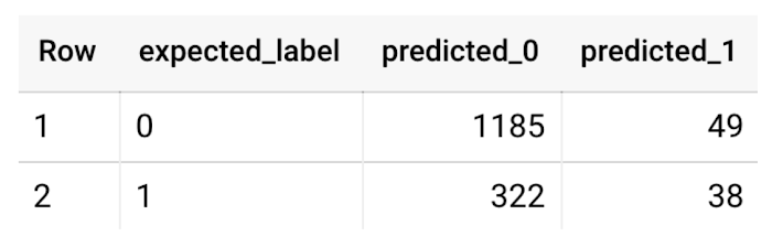
This table can be interpreted in the following way:

Make predictions using BigQuery ML
Once the ideal model was available, we ran ML.PREDICT to make predictions. For propensity modeling, the most important output is the probability of a behavior occurring. The following query returns the probability that the user will return after 24 hrs. The higher the probability and closer it is to 1, the more likely the user is predicted to return, and the closer it is to 0, the more likely the user is predicted to churn.
SELECTuser_pseudo_id,returned,predicted_returned,predicted_returned_probs[OFFSET(0)].prob as probability_returnedFROMML.PREDICT(MODEL bqmlga4.churn_logreg,(SELECT * FROM bqmlga4.train)) #can be replaced with a proper test dataset
Utilize predictions for activation
Once the model predictions are available for your users, you can activate this insight in different ways. In our analysis, we used user_pseudo_id as the user identifier. However, ideally, your app should send back the user_id from your app to Google Analytics. In addition to using first-party data for model predictions, this will also let you join back the predictions from the model into your own data.
- You can import the model predictions back into Google Analytics as a user attribute. This can be done using the Data Import feature for Google Analytics 4. Based on the prediction values you can Create and edit audiences and also do Audience targeting. For example, an audience can be users with prediction probability between 0.4 and 0.7, to represent users who are predicted to be “on the fence” between churning and returning.
- For Firebase Apps, you can use the Import segments feature. You can tailor user experience by targeting your identified users through Firebase services such as Remote Config, Cloud Messaging, and In-App Messaging. This will involve importing the segment data from BigQuery into Firebase. After that you can send notifications to the users, configure the app for them, or follow the user journeys across devices.
- Run targeted marketing campaigns via CRMs like Salesforce, e.g. send out reminder emails.
You can find all of the code used in this blogpost in the Github repository:
What’s next?
Continuous model evaluation and re-training
As you collect more data from your users, you may want to regularly evaluate your model on fresh data and re-train the model if you notice that the model quality is decaying.
Continuous evaluation—the process of ensuring a production machine learning model is still performing well on new data—is an essential part in any ML workflow. Performing continuous evaluation can help you catch model drift, a phenomenon that occurs when the data used to train your model no longer reflects the current environment.
To learn more about how to do continuous model evaluation and re-train models, you can read the blogpost: Continuous model evaluation with BigQuery ML, Stored Procedures, and Cloud Scheduler
More resources
If you’d like to learn more about any of the topics covered in this post, check out these resources:
- BigQuery export of Google Analytics data
- BigQuery ML quickstart
- Events automatically collected by Google Analytics 4
- Qwiklabs: Create ML models with BigQuery ML
Or learn more about how you can use BigQuery ML to easily build other machine learning solutions:
- How to build demand forecasting models with BigQuery ML
- How to build a recommendation system on e-commerce data using BigQuery ML
Let us know what you thought of this post, and if you have topics you’d like to see covered in the future! You can find us on Twitter at @polonglin and @_mkazi_.Thanks to reviewers: Abhishek Kashyap, Breen Baker, David Sabater Dinter.
How to Pick a Database that is Suitable for Your Application

7056
Of your peers have already read this article.
2:30 Minutes
The most insightful time you'll spend today!
Picking the right database for your application is not easy. The choice depends heavily on your use case—transactional processing, analytical processing, in-memory database, and so on—but it also depends on other factors. This post covers the different database options available within Google Cloud across relational (SQL) and non-relational (NoSQL) databases and explains which use cases are best suited for each database option.

Relational databases
In relational databases information is stored in tables, rows and columns, which typically works best for structured data. As a result they are used for applications in which the structure of the data does not change often. SQL (Structured Query Language) is used when interacting with most relational databases. They offer ACID consistency mode for the data, which means:
- Atomic: All operations in a transaction succeed or the operation is rolled back.
- Consistent: On the completion of a transaction, the database is structurally sound.
- Isolated: Transactions do not contend with one another. Contentious access to data is moderated by the database so that transactions appear to run sequentially.
- Durable: The results of applying a transaction are permanent, even in the presence of failures.
Because of these properties, relational databases are used in applications that require high accuracy and for transactional queries such as financial and retail transactions. For example: In banking when a customer makes a funds transfer request, you want to make sure the transaction is possible and it actually happens on the most up-to-date account balance, in this case an error or resubmit request is likely fine.
There are three relational database options in Google Cloud: Cloud SQL, Cloud Spanner, and Bare Metal Solution.
Cloud SQL: Provides managed MySQL, PostgreSQL and SQL Server databases on Google Cloud. It reduces maintenance cost and automates database provisioning, storage capacity management, back ups, and out-of-the-box high availability and disaster recovery/failover. For these reasons it is best for general-purpose web frameworks, CRM, ERP, SaaS and e-commerce applications.
Cloud Spanner: Cloud Spanner is an enterprise-grade, globally-distributed, and strongly-consistent database that offers up to 99.999% availability, built specifically to combine the benefits of relational database structure with non-relational horizontal scale. It is a unique database that combines ACID transactions, SQL queries, and relational structure with the scalability that you typically associate with non-relational or NoSQL databases. As a result, Spanner is best used for applications such as gaming, payment solutions, global financial ledgers, retail banking and inventory management that require ability to scale limitlessly with strong-consistency and high-availability.
Bare Metal Solution: Provides hardware to run specialized workloads with low latency on Google Cloud. This is specifically useful if there is an Oracle database that you want to lift and shift into Google Cloud. This enables data center retirements and paves a path to modernize legacy applications.
Non-relational databases
Non-relational databases (or NoSQL databases) store compex, unstructured data in a non-tabular form such as documents. Non-relational databases are often used when large quantities of complex and diverse data need to be organized. Unlike relational databases, they perform faster because a query doesn’t have to access several tables to deliver an answer, making them ideal for storing data that may change frequently or for applications that handle many different kinds of data.
For example, an apparel store might have a database in which shirts have their own document containing all of their information, including size, brand, and color with room for adding more parameters later such as sleeve size, collars, and so on.
Qualities that make NoSQL databases fast:
- Eventual consistency: stores usually exhibit consistency at some later point (e.g., lazily at read time)
- Horizontal scaling, usually using hashed distributions
- Typically, they are optimized for a specific workload pattern (i.e., key-value, graph, wide-column)
- Typically, they don’t support cross shard transactions or flexible isolation modes.
Because of these properties, non-relational databases are used in applications that require large scale, reliability, availability, and frequent data changes.They can easily scale horizontally by adding more servers, unlike some relational databases, which scale vertically by increasing the machine size as the data grows. Although, some relations databases such as Cloud Spanner support scale-out and strict consistency.
Non-relational databases can store a variety of unstructured data such as documents, key-value, graphs, wide columns, and more. Here are your non-relational database options in Google Cloud:
- Document databases: Store information as documents (in formats such as JSON and XML). For example: Firestore
- Key-value stores: Group associated data in collections with records that are identified with unique keys for easy retrieval. Key-value stores have just enough structure to mirror the value of relational databases while still preserving the benefits of NoSQL. For example: Datastore, Bigtable, Memorystore
- In-memory database: Purpose-built database that relies primarily on memory for data storage. These are designed to attain minimal response time by eliminating the need to access disks. They are ideal for applications that require microsecond response times and can have large spikes in traffic. For example: Memorystore
- Wide-column databases: Use the tabular format but allow a wide variance in how data is named and formatted in each row, even in the same table. They have some basic structure while preserving a lot of flexibility. For example: Bigtable
- Graph databases: Use graph structures to define the relationships between stored data points; useful for identifying patterns in unstructured and semi-structured information. For example: JanusGraph
There are three non-relational databases in Google Cloud:
- Firestore: Is a serverless document database which scales on demand and acts as a backend-as-a-service. It is DBaaS that increases the speed of building applications. It is perfect for all general purpose uses cases such as ecommerce, gaming, IoT and real time dashboards. With Firestore users can interact with and collaborate on live and offline data making it great for real-time application and mobile apps.
- Cloud Bigtable: Cloud Bigtable is a sparsely populated table that can scale to billions of rows and thousands of columns, enabling you to store terabytes or even petabytes of data. It is ideal for storing very large amounts of single-keyed data with very low latency. It supports high read and write throughput at sub-millisecond latency, and it is an ideal data source for MapReduce operations. It also supports the open-source HBase API standard to easily integrate with the Apache ecosystem including HBase, Beam, Hadoop and Spark along with Google Cloud ecosystem.
- Memorystore: Memorystore is a fully managed in-memory data store service for Redis and Memcached at Google Cloud. It is best for in-memory and transient data stores and automates the complex tasks of provisioning, replication, failover, and patching so you can spend more time coding. Because it offers extremely low latency and high performance, Memorystore is great for web and mobile, gaming, leaderboard, social, chat, and news feed applications.
Conclusion
Choosing a relational or a non-relational database largely depends on the use case. Broadly, if your application requires ACID transactions and your data structure is not going to change much, select a relational database.
In Google Cloud use Cloud SQL for any general-purpose SQL database and Cloud Spanner for large-scale globally scalable, strongly consistent use cases. In general, if your data structure may change later and if scale and availability is a bigger requirement than consistency then a non-relational database is a preferable choice. Google Cloud offers Firestore, Memorystore, and Cloud Bigtable to support a variety of use cases across the document, key-value, and wide column database spectrum.
For more comparison resources on each database check out the overview. For more hands-on experience with Bigtable, check out our on-demand training here and learn about migrating databases to managed services check out this whitepaper.
https://youtube.com/watch?v=2TZXSnCTd7E%3Fenablejsapi%3D1%26
For more #GCPSketchnote, follow the GitHub repo. For similar cloud content follow me on Twitter @pvergadia and keep an eye out on thecloudgirl.dev.
Bitly’s Big Move: A Story of Massive Data Migration to Google’s Cloud Bigtable
966
Of your peers have already read this article.
3:30 Minutes
The most insightful time you'll spend today!
Editor’s note: Bitly, the link & QR Code management platform, migrated 80 billion rows of link data to Cloud Bigtable. Here’s how and why they moved this data from a MySQL database, all in just six days.
Our goal at Bitly is simple: Make your life easier with connections. Whether you’re sharing links online, connecting the physical and digital worlds with custom QR Codes or creating a killer Link-in-bio, we’re here to help make that happen.
Bitly customers run the gamut from your local middle school to most of the Fortune 500 with every use case you can think of in play. On a typical day, we process approximately 360 million link clicks and QR Code scans and support the creation of 6-7 million links or QR Codes for more than 350,000 unique users.
At the heart of our platform is link data consisting of three major datasets for the approximately 40 billion active links in our system (and counting). For years we stored this data in a self-managed, manually sharded MySQL database. While that setup served us well over time, it did present some challenges as we looked to expand and move into the future.
MySQL: Challenges and growing pains
First, performing operational actions like software and security upgrades or database host provisioning — all while keeping the databases 100% available for our customers — was challenging to say the least.
Additionally, the backup and restore process was both costly and time-consuming. Daily backups for the growing dataset took almost an entire day to complete. And if we ever had to restore the entire data set, it would have undoubtedly taken at least two people working for several days — not a fun prospect and thankfully something we never had to do.
While manual sharding for MySQL offers good key distribution across physical and logical shards, it’s pretty high-maintenance — we tried to avoid touching our sharding config because of how error-prone making changes was. And even with a forward-thinking shard allocation, we found this approach to have a limited lifespan.
And finally, when we turned our attention towards multi-region and global distribution, manually sharded MySQL proved to be a major hurdle, especially compared to the convenience of a managed service that handles geo-distribution for us.
As we thought about the future of our data and how to best meet our expansion goals, we determined that an update was necessary. We needed a system more set up for growth and increased reliability, preferably one with built-in functionality for replication and scaling. Investigation and research brought us to Cloud Bigtable, Google Cloud’s enterprise-grade NoSQL database service.
The Bitly link, in a nutshell
Before we dive into the Bigtable migration, it’s useful to understand the basics of our link management system. When a user shortens a long URL with Bitly, information is saved to the backend data stores through our API layer. This information consists of a Bitly short link and the corresponding destination link for proper routing, as well as some additional metadata. When a user clicks the Bitly short link, our services query these same backend data stores for the redirect destination for the request. This basic flow, which also includes other Bitly link options like custom back-halves, is the backbone of the Bitly link management platform.
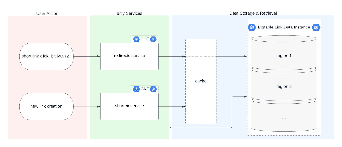
Where Bigtable comes in
As mentioned, after researching our options, the solution that best fit our needs was Bigtable. It offered the features we were looking for, including:
- A 99.999% SLA
- Limitless scale
- Single-digit millisecond latency
- A built-in monitoring system
- Multi-region replication
- Geo-distribution, which allows for seamless replication of data across regions and reduces latency
- On-demand scaling of compute resources and storage, which adjusts to user traffic and allows our system to grow and scale as needed
- Seamless integration with our general architecture; we use Google Cloud services for many other parts of our system, including the APIs that interact with these databases
- A NoSQL database that doesn’t require relational semantics, as the datasets we’re migrating are indexed on a single primary key in our applications
Making the move
We targeted three of our major, self-managed datasets to migrate. The larger two were organized in a sharded database architecture. The first thing we did for migration was prepare the new Bigtable database. We iterated over a schema design process and conducted a thorough performance analysis of Bigtable to ensure an uninterrupted user experience during and after the migration. After that, we made minor adjustments to our application code so that it could seamlessly integrate and interact with Bigtable. Finally, we implemented a robust post-migration disaster recovery process to mitigate any potential risks.
During the actual migration, we enabled our applications to start a “dual writes” phase. This involved concurrently writing new link data to both our existing MySQL and the new Bigtable tables. Once data started writing to our Bigtable instance, we ran our migration scripts. We used a Go script to walk each of the existing MySQL datasets and insert each row into Bigtable. This enabled us to clean up outdated information and backfill older records with newer field data.
Cleaning up clutter along the way
In the process of migration, we were actually able to free up a huge amount of storage. Because of the elimination of an early feature of the Bitly platform, we were able to exclude from the migration to Bigtable a little less than half of the total data stored in MySQL. Since we were creating a completely clean dataset, we had the opportunity simply to skip those unneeded rows during the migration.
Altogether, the migration process walked through 80 billion MySQL rows, which resulted in just over 40 billion records finding their new home in Bigtable. In the end, our starting point with Bigtable is a 26 TB dataset, not including replication. A set of concurrent Go scripts running in parallel on a handful of machines allowed us to complete this migration project in six days. (Go rarely disappoints.)
Write twice, cut once – validation before migration
Next up was the data validation and cutover period when we started returning data from Bigtable, but continued to write to MySQL as a precaution in case we needed to roll back at any point.
As we dove into the validation process, we compared the data between MySQL and Bigtable and noted any discrepancies whenever a link was clicked or created. After verifying that all our responses were stable, we proceeded with a gradual cutover process, rolling out in percentages until we reached 100% Bigtable for all writes and reads. After a comfortable run period, we’ll turn off the dual writes completely and finally decommission our workhorse MySQL hosts to live on a farm upstate.
Google’s got Bitly’s back(ups)
Our data is our lifeline, and we’re doing everything we can to ensure it’s always protected. We put together a redundancy plan using both Bigtable backups as well as a process for keeping a copy of the data outside Bigtable for true disaster recovery.
The first line of defense involves a switchover to the backup Bigtable dataset in case we need it. Beyond that, we’ve implemented two more layers of defense to protect against instance failure, corrupted data, and any other data failure that would require a restore of one or more tables from backup.
For this process, we start by creating daily Bigtable backups of our tables that we store for a fixed number of days. Second, we execute a Dataflow job to export our data from Bigtable into Cloud Storage approximately every week. And, if the need arises, we can use Dataflow to import our data back from Cloud Storage into a new Bigtable table.
While running the Dataflow jobs to export from Bigtable to Cloud Storage, we’ve seen an impressive export speed of 7-8 million rows read per second on average and up to 15 million per second at times. All the while, our production reads and writes continued without disruption. When we tested the Cloud-Storage-to-Bigtable restore job, the write speed, expectedly, increased with instance scale — at the maximum node quota for our regions, we observed an average of just under 2 million rows per second written to our new table.
Short links for the long haul
As mentioned above, not only did Bigtable meet our technical requirements and operational needs, but we also chose Bigtable because it sets us up for future growth. Its ability to scale seamlessly over time while improving our system availability SLA was a major factor in our decision.
As we increase our scale by 5x, 10x, or more, it’s imperative that our data backbone scales accordingly and that the SLAs we provide to customers stay stable or even add another coveted “9”. We have big plans in the coming years and Bigtable will help us achieve them.
Interested in learning more? We found the following resources to be useful in our journey to Bigtable evaluation and ultimate adoption:
- Evaluate Bigtable schema design for your relational database and application workloads
- Understand how to increase availability and distribute data globally with Bigtable replication in any region combination of your choice
- Learn more about Bigtable backups and importing/exporting data with Bigtable Dataflow templates
Bonus: If you’re interested in learning more of the nuts and bolts of how we migrated the data, I’ll be talking all about that very topic at GopherCon 2023 this September in San Diego!
More Relevant Stories for Your Company


What is Cloud Spanner and Is It the Right Database for You?
You’ve probably heard about Cloud Spanner, but what exactly does it do that is so different from other databases out there? How do you know if it’s worth spending your valuable time trying out? Cloud Spanner is the first enterprise-grade, globally distributed, and strongly consistent database service built for the

Dataflow Guarantees 50+% Increase in Developer Productivity and Infrastructure Cost Savings: Read More
In our conversations with technology leaders about data-driven transformation using Google Data Cloud - industry’s leading unified data and AI solution - , one important topic is incorporating continuous intelligence to move from answering questions such as “What has happened? to questions like “What is happening?” and “What might happen?”.

Optimizing Terabyte-scale PostgreSQL Migrations to Cloud SQL Using Searce
Google Cloud allows you to move your PostgreSQL databases to Cloud SQL with Database Migration Service (DMS). DMS gives you the ability to replicate data continuously to the destination database, while the source is live in production, enabling you to migrate with minimum downtime. However, terabyte-scale migrations can be complex.


How Apna is using data and AI to drive the gig economy in India
In this episode, Theo speaks to Ronak Shah, Head of Data at apna.co. As one of the largest gig economies in the world, India is seeing rising numbers among younger people joining the ecosystem. Driven by digital adoption and new ways of working, Apna saw an opportunity to help bridge
