





How to Enhance Incremental Pipeline Performance while Ingesting Data into BigQuery

6326
Of your peers have already read this article.
3:00 Minutes
The most insightful time you'll spend today!
When you build a data warehouse, the important question is how to ingest data from the source system to the data warehouse. If the table is small you can fully reload a table on a regular basis, however, if the table is large a common technique is to perform incremental table updates. This post demonstrates how you can enhance incremental pipeline performance when you ingest data into BigQuery.
Setting up a standard incremental data ingestion pipeline
We will use the below example to illustrate a common ingestion pipeline that incrementally updates a data warehouse table. Let’s say that you ingest data into BigQuery from a large and frequently updated table in the source system, and you have Staging and Reporting areas (datasets) in BigQuery.

The Reporting area in BigQuery stores the most recent, full data that has been ingested from the source system tables. Usually you create the base table as a full snapshot of the source system table. In our running example, we use BigQuery public data as the source system and create reporting.base_table as shown below. In our example each row is identified by a unique key which consists of two columns: block_hash and log_index.
CREATE TABLE reporting.base_table --156 GB processedPARTITION BY TIMESTAMP_TRUNC(block_timestamp, DAY) ASSELECT log_index, data, topics, block_timestamp, block_hashFROM bigquery-public-data.crypto_ethereum.logsWHERE block_timestamp BETWEEN TIMESTAMP '2020-01-01' AND TIMESTAMP '2020-11-30';
In data warehouses it is common to partition a large base table by a datetime column that has a business meaning. For example, it may be a transaction timestamp, or datetime when some business event happened, etc. The idea is that data analysts who use the data warehouse usually need to analyze only some range of dates and rarely need the full data. In our example, we partition the base table by block_timestamp which comes from the source system.
After ingesting the initial snapshot you need to capture changes that happen in the source system table and update the reporting base table accordingly. This is when the Staging area comes into the picture. The staging table will contain captured data changes that you will merge into the base table. Let’s say that in our source system on a regular basis we have a set of new rows and also some updated records. In our example we mock the staging data as follows: first, we create new data, than we mock the updated records:
CREATE TABLE staging.load_delta AS --5 GB processedSELECT log_index, data, topics, block_timestamp, block_hashFROM bigquery-public-data.crypto_ethereum.logsWHERE block_timestamp BETWEEN TIMESTAMP '2020-12-01' AND TIMESTAMP '2020-12-07';INSERT INTO staging.load_delta --2 GB processedSELECT log_index, CONCAT(data, RAND()), topics, block_timestamp, block_hashFROM bigquery-public-data.crypto_ethereum.logs TABLESAMPLE SYSTEM (5 PERCENT)WHERE block_timestamp BETWEEN TIMESTAMP '2020-10-01' AND TIMESTAMP '2020-11-30';
Next, the pipeline merges the staging data into the base table. It joins two tables by unique key and than updates the changed value or inserts a new row
MERGE INTO reporting.base_table T --161 GB processedUSING staging.load_delta SON T.block_hash = S.block_hashAND T.log_index = S.log_indexWHEN MATCHED THEN UPDATE SETT.data = S.dataWHEN NOT MATCHED THEN INSERT (log_index, data, topics, block_timestamp, block_hash)VALUES (log_index, data, topics, block_timestamp, block_hash);
It is often the case that the staging table contains keys from various partitions but the number of those partitions are relatively small. It holds, for instance, because in the source system the recently added data may get changed due to some initial errors or ongoing processes but older records are rarely updated. However, when the above MERGE gets executed, BigQuery scans all partitions in the base table and processes 161 GB of data. You might add additional join condition on block_timestamp:
MERGE INTO reporting.base_table T --161 GB processedUSING staging.load_delta SON T.block_hash = S.block_hashAND T.log_index = S.log_indexAND T.block_timestamp = S.block_timestampWHEN MATCHED THEN UPDATE SETT.data = S.dataWHEN NOT MATCHED THEN INSERT (log_index, data, topics, block_timestamp, block_hash)VALUES (log_index, data, topics, block_timestamp, block_hash);
But BigQuery would still scan all partitions in the base table because condition T.block_timestamp = S.block_timestamp is a dynamic predicate and BigQuery doesn’t automatically push such predicates down from one table to another in MERGE.
Can you improve the MERGE efficiency by making it scan less data? The answer is Yes.
As described in the MERGE documentation, pruning conditions may be located in a subquery filter, a merge_condition filter, or a search_condition filter. In this post we show how you can leverage the first two. The main idea is to turn a dynamic predicate into a static predicate.
Steps to enhance your ingestion pipeline
The initial step is to compute the range of partitions that will be updated during the MERGE and store it in a variable. As was mentioned above, in data ingestion pipelines, staging tables are usually small so the cost of the computation is relatively low.
DECLARE src_range STRUCT<date_min TIMESTAMP, date_max TIMESTAMP> --115 MB processedDEFAULT(SELECT STRUCT(MIN(block_timestamp) AS date_min,MAX(block_timestamp) AS date_max) FROM staging.load_delta);
Based on your existing ETL/ELT pipeline, you can add the above code as-is to your pipeline or you can compute date_min, data_max as part of some already existing transformation step. Alternatively, date_min, data_max can be computed on the Source System side while capturing the next ingestion data batch.
After computing date_min, date_max you pass those values to the MERGE statement as static predicates. There are several ways to enhance the MERGE and prune partitions in the base table based on precomputed date_min, data_max.
If your initial MERGE statement uses a subquery, you can incorporate a new filter into it:
BEGINDECLARE src_range STRUCT<date_min TIMESTAMP, date_max TIMESTAMP> --115 MB processedDEFAULT(SELECT STRUCT(MIN(block_timestamp) AS date_min,MAX(block_timestamp) AS date_max) FROM staging.load_delta);MERGE INTO reporting.base_table T --41 GB processedUSING (SELECT *FROM staging.load_deltaWHERE block_timestamp BETWEEN src_range.date_min AND src_range.date_max) SON T.block_hash = S.block_hashAND T.log_index = S.log_indexAND T.block_timestamp = S.block_timestampWHEN MATCHED THEN UPDATE SETT.data = S.dataWHEN NOT MATCHED THEN INSERT (log_index, data, topics, block_timestamp, block_hash)VALUES (log_index, data, topics, block_timestamp, block_hash);END;
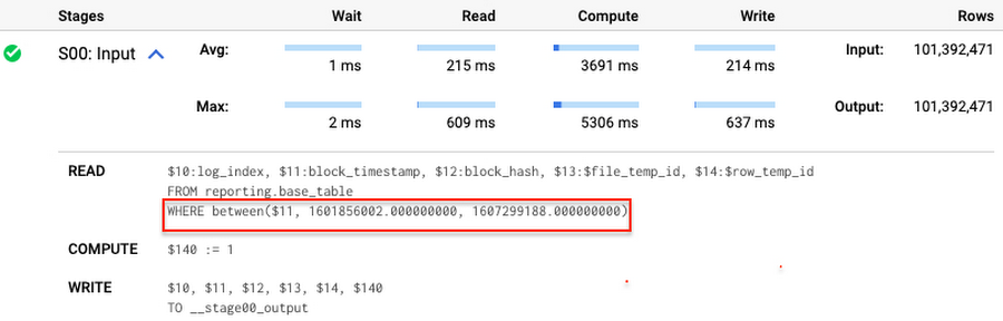
Note that you add the static filter to the staging table and keep T.block_timestamp = S.block_timestamp to convey to BigQuery that it can push that filter to the base table. This MERGE processes 41 GB of data in contrast to the initial 161 GB. You can see in the query plan that BigQuery pushes the partition filter from the staging table to the base table:
This type of optimization, when a pruning condition is pushed from a subquery to a large partitioned or clustered table, is not unique for MERGE. It also works for other types of queries. For instance:
SELECT * -- 41 GB processedFROM reporting.base_table TINNER JOIN staging.load_delta SON T.block_hash = S.block_hashAND T.log_index = S.log_indexAND T.block_timestamp = S.block_timestampWHERE S.block_timestamp BETWEEN TIMESTAMP '2020-10-05' AND TIMESTAMP '2020-12-07'
And you can check the query plan to verify that BigQuery pushed down the partition filter from one table to another.
Moreover, for SELECT statements, BigQuery can automatically infer a filter predicate on a join column and push it down from one table to another if your query meets the following criteria:
- The target table must be clustered or partitioned.
- The result size of the other table, i.e. after applying all filters, must qualify for broadcast join. Namly, the result set must be relatively small, less than ~100MB.
In our running example, reporting.base_table is partitioned by block_timestamp. If you define a selective filter on staging.load_delta and join two tables, you can see an inferred filter on the join key pushed to the target table
SELECT *FROM reporting.base_table TINNER JOIN staging.load_delta SON T.block_timestamp = S.block_timestampWHERE S.block_hash = '0x0c1caa16b34d94843aabfebc0d5a961db358135988f7498a6fdc450ad55f0870'
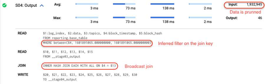
There is no requirement to join tables by partitioning or clustering key to kick off this type of optimization. However, in this case the pruning effect on the target table would be less significant.
But let us get back to the pipeline optimizations. Another way to enhance MERGE is to modify the merge_condition filter by adding static predicate on the base table:
BEGINDECLARE src_range STRUCT<date_min TIMESTAMP, date_max TIMESTAMP> --115 MB processedDEFAULT(SELECT STRUCT(MIN(block_timestamp) AS date_min,MAX(block_timestamp) AS date_max) FROM staging.load_delta);MERGE INTO reporting.base_table T --41 GB processedUSING staging.load_delta SON T.block_hash = S.block_hashAND T.log_index = S.log_indexAND T.block_timestamp BETWEEN src_range.date_min AND src_range.date_maxWHEN MATCHED THEN UPDATE SETT.data = S.dataWHEN NOT MATCHED THEN INSERT (log_index, data, topics, block_timestamp, block_hash)VALUES (log_index, data, topics, block_timestamp, block_hash);END;
To summarize, here are the steps that you can perform to enhance incremental ingestion pipelines in BigQuery. First you compute the range of updated partitions based on the small staging table. Next, you tweak the MERGE statement a bit to let BigQuery know to prune data in the base table.
All the enhanced MERGE statements scanned 41 GB of data, and setting up the src_range variable took 115 MB. Compare it with the initial 161 GB scan. Moreover, given that computing src_range may be incorporated into some existing transformation in your ETL/ELT, it results in a good performance improvement which you can leverage in your pipelines.
In this post we described how to enhance data ingestion pipelines by turning dynamic filter predicates into static predicates and letting BiQuery prune data for us. You can find more tips on BigQuery DML tuning here.
Special thanks to Daniel De Leo, who helped with examples and provided valuable feedback on this content.
How BigQuery’s Unique Features Support Your Data at Petabyte-scale

4793
Of your peers have already read this article.
3:00 Minutes
The most insightful time you'll spend today!
Organizations rely on data warehouses to aggregate data from disparate sources, process it, and make it available for data analysis in support of strategic decision-making. BigQuery is the Google Cloud enterprise data warehouse designed to help organizations to run large scale analytics with ease and quickly unlock actionable insights. You can ingest data into BigQuery either through batch uploading or by streaming data directly to unlock real-time insights. As a fully-managed data warehouse, BigQuery takes care of the infrastructure so you can focus on analyzing your data up to petabyte-scale. BigQuery supports SQL (Structured Query Language), which you’re likely already familiar with if you’ve worked with ANSI-compliant relational databases.
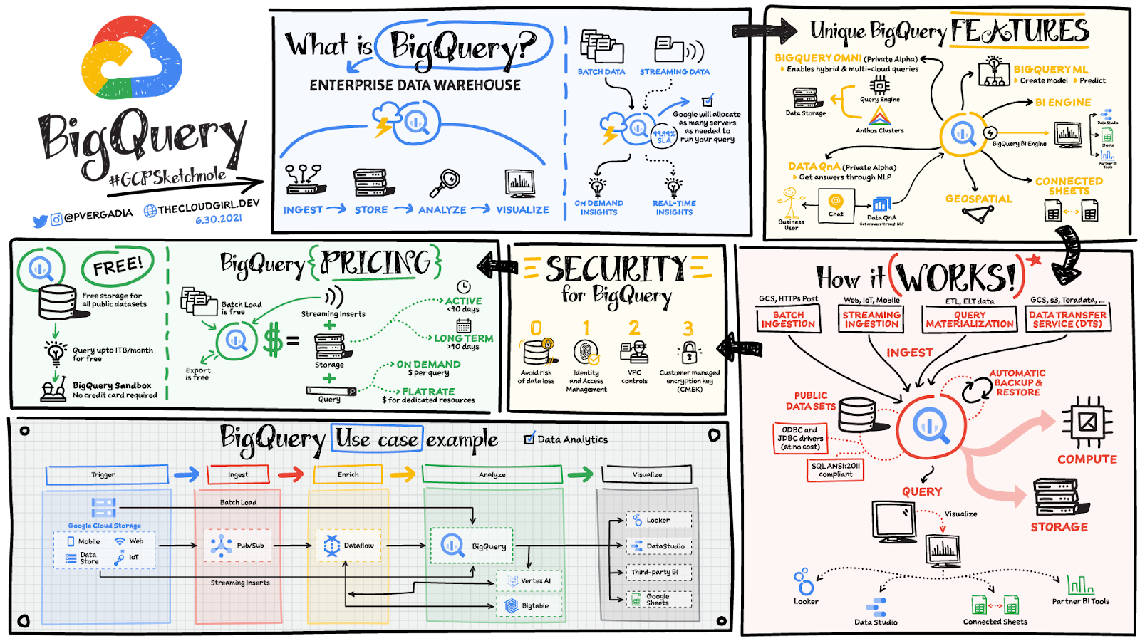
BigQuery unique features
BI Engine – BigQuery BI Engine is a fast, in-memory analysis service that provides subsecond query response times with high concurrency. BI Engine integrates with Google Data Studio and Looker for visualizing query results and enables integration with other popular business intelligence (BI) tools.
BigQuery ML: BigQuery ML is unlocking machine learning for millions of data analysts. It enables data analysts and data scientists to build and operationalize machine learning models directly within BigQuery, using simple SQL.
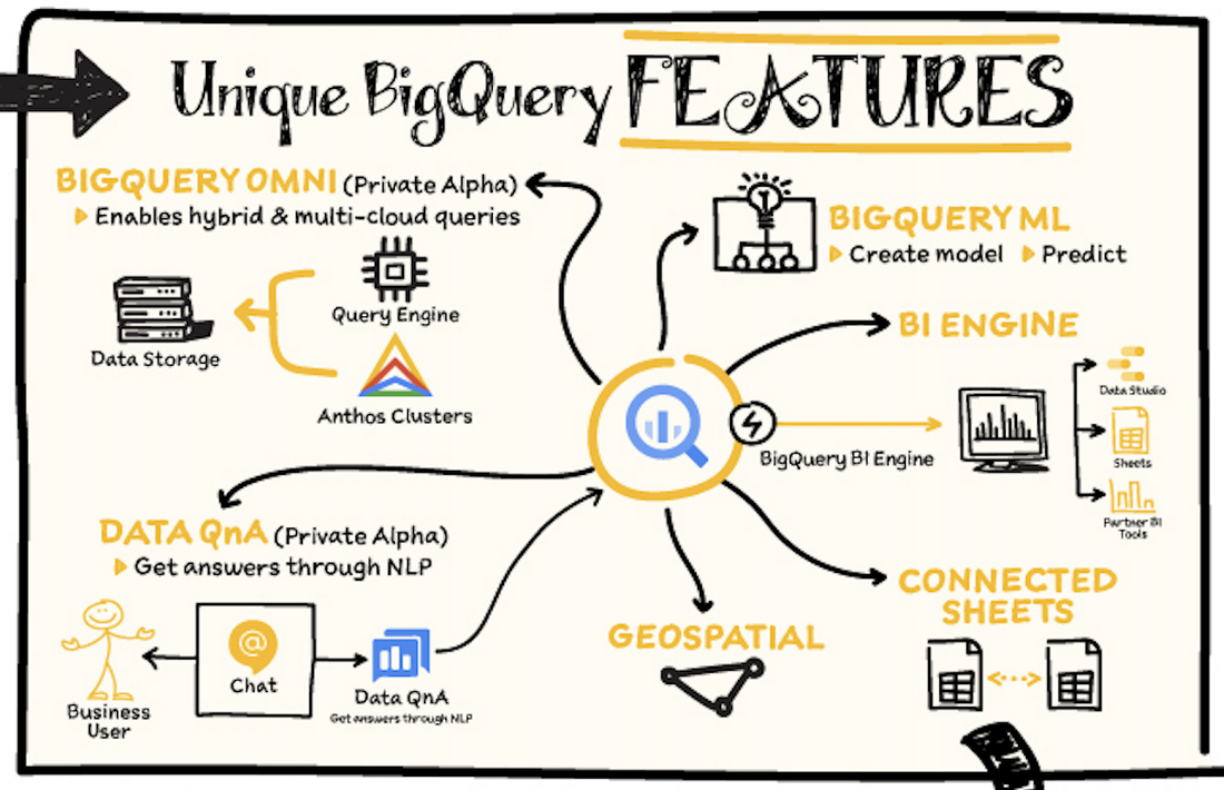
BigQuery Omni – BigQuery Omni is a flexible, multi-cloud analytics solution powered by Anthos that lets you cost-effectively access and securely analyze data across Google Cloud, Amazon Web Services (AWS), and Azure, without leaving the BigQuery user interface (UI). Using standard SQL and familiar BigQuery APIs, you can break down data silos and gain critical business insights from a single pane of glass.
Data QnA: Data QnA enables self-service analytics for business users on BigQuery data as well as federated data from Cloud Storage, Bigtable, Cloud SQL, or Google Drive. It uses Dialogflow and enables users to formulate free-form text analytical questions, with auto-suggested entities while users type a question.
Connected Sheets -The native integration between Sheets and BigQuery makes it possible for all business stakeholders, who are already quite familiar with spreadsheet tools, to get their own up-to-date insights at any time.
Geospatial data – BigQuery offers accurate and scalable geospatial analysis with geography data types. It supports core GIS functions – measurements, transforms, constructors, and more – using standard SQL.
How does it work?
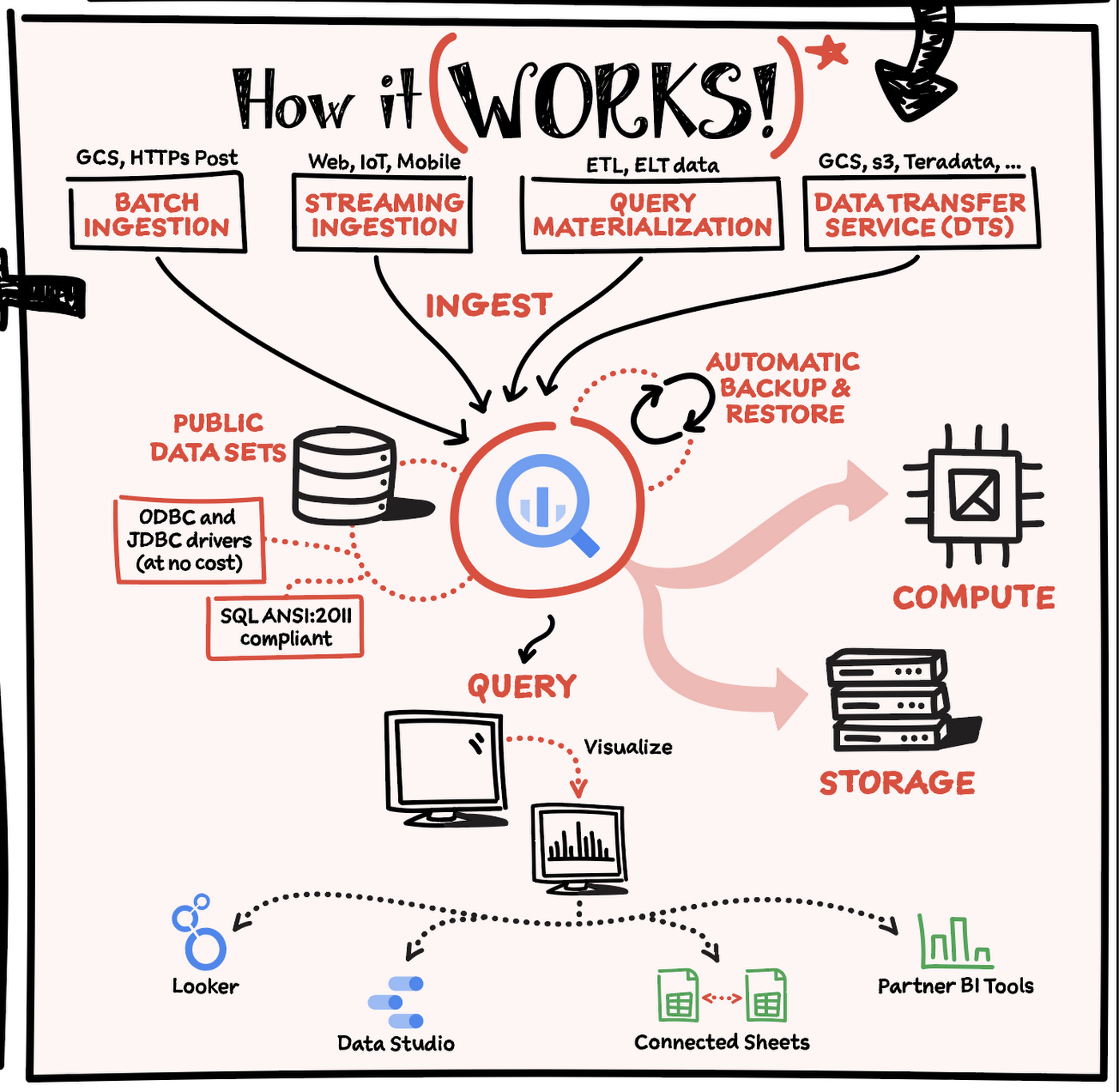
Here’s how it works: You ingest your own data into BigQuery or use data from the public datasets. Storage and compute are decoupled and can scale independently on demand. This offers immense flexibility and cost control for your business as you don’t need to keep expensive compute resources up and running all the time. As a result, BigQuery is much more cost-effective than traditional node-based cloud data warehouse solutions or on-premises systems. BigQuery also provides automatic backup and restore of your data.
You can ingest data into BigQuery in batches or stream real-time data from web, IoT, or mobile devices via Pub/Sub. You can also use Data Transfer Service to ingest data from other clouds, on-premises systems or third-party services. BigQuery also supports ODBC and JDBC drivers to connect with existing tools and infrastructure.
Interacting with BigQuery to load data, run queries, or create ML models can be done in three different ways. You can use the UI in the Cloud Console, the BigQuery command-line tool, or the API via client libraries available in several languages.
When it comes time to visualize your data, BigQuery integrates with Looker as well as several other business intelligence tools across the Google partner ecosystem.
What about security?
BigQuery offers built-in data protection at scale. It provides security and governance tools to efficiently govern data and democratize insights within your organization.
- Within BigQuery, users can assign dataset-level and project-level permissions to help govern data access. Secure data sharing ensures you can collaborate and operate your business with trust.
- Data is automatically encrypted both while in transit and at rest, ensuring that your data is protected from intrusions, theft, and attacks.
- Cloud DLP helps you discover and classify sensitive data assets.
- Cloud IAM provides access control and visibility into security policies.
- Data Catalog helps you discover and manage data.
How much does it cost?
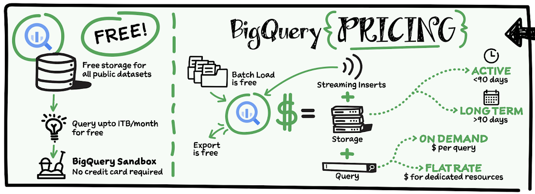
The BigQuery sandbox lets you explore BigQuery capabilities at no cost and confirm that BigQuery fits your needs. With BigQuery you get predictable price-performance: you pay for storing and querying data, and for streaming inserts. Loading and exporting data are free of charge. Storage costs are based on the amount of data stored, and have two rates based on how often the data is changing. Query costs can be either:
- On-demand – you are charged per query by the amount of data processed
- Flat-rate – if you prefer to purchase dedicated resources
You can start with the pay-as-you-go, on-demand option and later move to flat-rate if that better suits your usage. Or, start with flat-rate, get a better understanding of your usage and move to the pay-as-you-go models for additional workloads.
To explore BigQuery and its capabilities a bit more, check out the sandbox; and when you’re ready to modernize your data warehouse with BigQuery then check out the documentation to streamline your migration process here. https://www.youtube.com/embed/So-tVyBQt8E?enablejsapi=1&
For more #GCPSketchnote, follow the GitHub repo. For similar cloud content follow me on Twitter @pvergadia and keep an eye out on thecloudgirl.dev.
Scaling Ad Personalization with Bigtable

2999
Of your peers have already read this article.
2:30 Minutes
The most insightful time you'll spend today!
Cloud Bigtable is a popular and widely used key-value database available on Google Cloud. The service provides scale elasticity, cost efficiency, excellent performance characteristics, and 99.999% availability SLA. This has led to massive adoption with thousands of customers trusting Bigtable to run a variety of their mission-critical workloads.
Bigtable has been in continuous production usage at Google for more than 15 years now. It processes more than 5 billion requests per second at peak and has more than 10 exabytes of data under management. It’s one of the largest semi-structured data storage services at Google.
One of the key use cases for Bigtable at Google is ad personalization. This post describes the central role that Bigtable plays within ad personalization.
Ad personalization
Ad personalization aims to improve user experience by presenting topical and relevant ad content. For example, I often watch bread-making videos on YouTube. If ads personalization is enabled in my ad settings, my viewing history could indicate to YouTube that I’m interested in baking as a topic and would potentially be interested in ad content related to baking products.
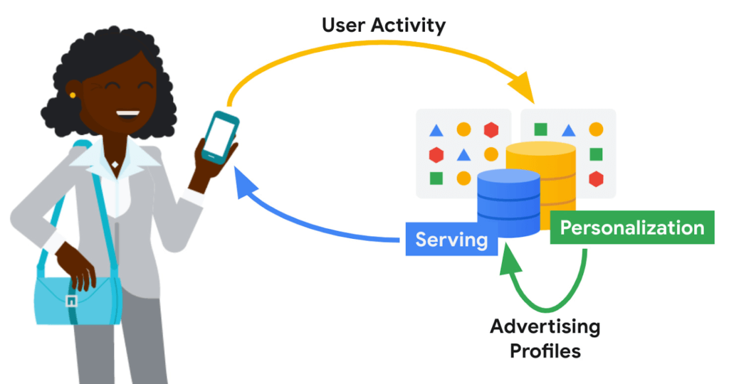
Ad personalization requires large-scale data processing in near real-time for timely personalization with strict controls for user data handling and retention. System availability needs to be high, and serving latencies need to be low due to the narrow window within which decisions need to be made on what ad content to retrieve and serve. Sub-optimal serving decisions (e.g. falling back to generic ad content) could potentially impact user experience. Ad economics requires infrastructure costs to be kept as low as possible.
Google’s ad personalization platform provides frameworks to develop and deploy machine learning models for relevance and ranking of ad content. The platform supports both real-time and batch personalization. The platform is built using Bigtable, allowing Google products to access data sources for ads personalization in a secure manner that is both privacy and policy compliant, all while honoring users’ decisions about what data they want to provide to Google
The output from personalization pipelines, such as advertising profiles are stored back in Bigtable for further consumption. The ad serving stack retrieves these advertising profiles to drive the next set of ad serving decisions.
Some of the storage requirements of the personalization platform include:
- Very high throughput access for batch and near real-time personalization
- Low latency (<20 ms at p99) lookup for reads on the critical path for ad serving
- Fast (i.e. in the order of seconds) incremental update of advertising models in order to reduce personalization delay
Bigtable
Bigtable’s versatility in supporting both low-cost, high-throughput access to data for offline personalization as well as consistent low-latency access for online data serving makes it an excellent fit for the ads workloads.
Personalization at Google-scale requires a very large storage footprint. Bigtable’s scalability, performance consistency and low cost required to meet a given performance curve are key differentiators for these workloads.
Data model
The personalization platform stores objects in Bigtable as serialized protobufs keyed by Object ids. Typical data sizes are less than 1 MB and serving latency is less than 20 ms at p99.
Data is organized as corpora, which correspond to distinct categories of data. A corpus maps to a replicated Bigtable.
Within a corpus, data is organized as DataTypes, logical groupings of data. Features, embeddings, and different flavors of advertising profiles are stored as DataTypes, which map to Bigtable column families. DataTypes are defined in schemas which describe the proto structure of the data and additional metadata indicating ownership and provenance. SubTypes map to Bigtable columns and are free-form.
Each row of data is uniquely identified by a RowID, which is based on the Object ID. The personalization API identifies individual values by RowID (row key), DataType (column family), SubType (column part), and Timestamp.
Consistency
The default consistency mode for operations is eventual. In this mode, data from the Bigtable replica nearest to the user is retrieved, providing the lowest median and tail latency.
Reads and writes to a single Bigtable replica are consistent. If there are multiple replicas of Bigtable in a region, traffic spillover across regions is more likely. To improve the likelihood of read-after-write consistency, the personalization platform uses a notion of row affinity. If there are multiple replicas in a region, one replica is preferentially selected for any given row, based on a hash of the Row ID.
For lookups with stricter consistency requirements, the platform first attempts to read from the nearest replica and requests that Bigtable return the current low watermark (LWM) for each replica. If the nearest replica happens to be the replica where the writes originated, or if the LWMs indicate that replication has caught up to the necessary timestamp, then the service returns a consistent response. If replication has not caught up, then the service issues a second lookup—this one targeted at the Bigtable replica where writes originated. That replica could be distant and the request could be slow. While waiting for a response, the platform may issue failover lookups to other replicas in case replication has caught up at those replicas.
Bigtable replication
The Ads personalization workloads use a Bigtable replication topology with more than 20 replicas, spread across four continents.
Replication helps address the high availability needs for ad serving. Bigtable’s zonal monthly uptime percentage is in excess of 99.9%, and replication coupled with a multi-cluster routing policy allows for availability in excess of 99.999%.
A globe-spanning topology allows for data placement that is close to users, minimizing serving latencies. However, it also comes with challenges such as variability in network link costs and throughputs. Bigtable uses Minimum Spanning Tree-based routing algorithms and bandwidth-conserving proxy replicas to help reduce network costs.
For ads personalization, reducing Bigtable replication delay is key to lowering the personalization delay (the time between a user’ action and when that action has been incorporated into advertising models to show more relevant ads to the user). Faster replication is preferred but we also need to balance serving traffic against replication traffic and make sure low-latency user-data serving is not disrupted due to incoming or outgoing replication traffic flows. Under the hood, Bigtable implements complex flow control and priority boost mechanisms to manage global traffic flows and to balance serving and replication traffic priorities.
Workload Isolation
Ad personalization batch workloads are isolated from serving workloads by pinning a given set of workloads onto certain replicas; some Bigtable replicas exclusively drive personalization pipelines while others drive user-data serving. This model allows for a continuous and near real-time feedback loop between serving systems and offline personalization pipelines, while protecting the two workloads from contending with each other.
For Cloud Bigtable users, AppProfiles and cluster-routing policies provide a way to confine and pin workloads to specific replicas to achieve coarse-grained isolation.
Data residency
By default, data is replicated to every replica—often spread out globally—which is wasteful for data that is only accessed regionally. Regionalization saves on storage and replication costs by confining data to the region where it is most likely to be accessed. Compliance with regulations mandating that data pertaining to certain subjects are physically stored within a given geographical area is also vital.
The location of data can be either implicitly determined by the access location of requests or through location metadata and other product signals. Once the location for a user is determined, it is stored in a location metadata table which points to the Bigtable replicas that read requests should be routed to. Migration of data based on row-placement policies happens in the background, without downtime or serving performance regressions.
Conclusion
In this blog post, we looked at how Bigtable is used within Google to support an important use case—modeling user intent for ad personalization.
Over the past decade, Bigtable has scaled as Google’s personalization needs have scaled by orders of magnitude. For large-scale personalization workloads, Bigtable offers low cost storage with excellent performance characteristics. It seamlessly handles global traffic flows with simple user configurations. Its ease at handling both low-latency serving and high-throughput batch computations make it an excellent option for lambda-style data processing pipelines.
We continue to drive high levels of investment to further lower costs, improve performance, and bring new features to make Bigtable an even better choice for personalization workloads.
Learn more
To get started with Bigtable, try it out with a Qwiklab and learn more about the product here.
Acknowledgements
We’d like to thank Ashish Awasthi, Ashish Chopra, Jay Wylie, Phaneendhar Vemuru, Bora Beran, Elijah Lawal, Sean Rhee and other Googlers for their valuable feedback and suggestions.
“It’s an Astonishing Difference”: What Data Operation Execs say About Google Cloud’s Data Warehouse

5651
Of your peers have already read this article.
8:30 Minutes
The most insightful time you'll spend today!
The popularity of meal kit delivery services has surged in recent years as consumer attitudes toward home cooking and grocery shopping have shifted. As a pioneer in the category, Blue Apron helps its customers create incredible home cooking experiences by sending culinary-driven recipes with high-quality ingredients and step-by-step instructions straight to customers’ doors. Blue Apron also offers a monthly wine subscription service and a la carte culinary tools and products through its marketplace.
If that sounds simple, it isn’t.
Ingredients for the meal kits must be sourced at the right time, quality, and price. Orders must be packed efficiently and in exactly the right proportions. Most importantly, meal kits must be delivered to the customer fresh and on time.
To meet these criteria and make data meaningful and intuitive to its managers, one of the tools Blue Apron relies on is Looker, an analytics platform that lets business users explore data and ask sophisticated questions using familiar terms. Looker integrates its solution with Google Cloud Platform to help customers modernize their analytics.
“The combination of Looker and Google BigQuery is powerful, allowing us to get data-hungry analysts essential information much faster. Because we choose to pay by the query, it’s also flexible and cost effective—plus storage is cheap, so we can just put data in and query what we need.”
—Sam Chase, Tech Lead, Data Operations, Blue Apron
Blue Apron previously used Looker with a single database instance hosted on another cloud provider. As data volumes grew and queries became more complex, it became difficult to scale. Blue Apron’s only options were choosing ever-larger server classes and increasing storage throughput by purchasing a higher number of provisioned IOPS. To improve speed, scalability, and cost efficiency, Blue Apron moved its data warehouse to Google BigQuery.
“The combination of Looker and Google BigQuery is powerful, allowing us to get data-hungry analysts essential information much faster,” says Sam Chase, Tech Lead, Data Operations at Blue Apron. “Because we choose to pay by the query, it’s also flexible and cost effective—plus storage is cheap, so we can just put data in and query what we need.”
“After we moved to Google BigQuery, query time was reduced exponentially. It’s an astonishing difference, allowing us to run 300 queries per day.”
—Sam Chase, Tech Lead, Data Operations, Blue Apron
The analytics platform of the future
When you’re making business decisions about a customer’s dinner, speed matters. Looker takes full advantage of the power of Google BigQuery, making it easy to build a data exploration platform.
Blue Apron’s applications publish event data to Kafka—approximately 140 million events per day—and data is then streamed into Google BigQuery, which performs lightning-fast queries on both streamed and static data. Now, business users and analytics teams can make decisions based on near real-time information in Looker, instead of waiting until the next business day for results.
“After we moved to Google BigQuery, query time was reduced exponentially. It’s an astonishing difference, allowing us to run 300 queries per day,” says Sam.
Previously, Blue Apron spent up to a week out of every month optimizing its data warehouse to attempt to improve query performance. With Google BigQuery, all maintenance is handled by Google, reclaiming 25% of up to two engineers’ time. Even when multiple people are using Looker concurrently, query performance never degrades and storage never runs out.
“Because Google BigQuery is architected as a giant, shared cluster, growth is smooth,” says Lloyd Tabb, Founder and CTO of Looker. “Like a race car going from 0 to 120 mph, there are no shift points, just smooth acceleration. To us, it looks like the future.”
An empowering, integrated toolset
Looker takes advantage of aggressive caching and support for date-based table partitioning in Google BigQuery to increase performance, simplify the load process, and improve data manageability. By partitioning data by time, Blue Apron can also take advantage of better long-term storage pricing without sacrificing query performance. When using Google BigQuery with Looker, analysts can easily see how much data is going to be scanned before each query is run.
Blue Apron is also using Looker for Google BigQuery Data Transfer Service to provide actionable analytics for all of the company’s Google marketing data from Google AdWords and DoubleClick by Google in one place to understand campaign performance across channels, saving its data operations team months of work. Using Looker Blocks, marketers can quickly make sense of the data with reports and dashboards, and set alerts when campaign performance hits certain thresholds.
“Everyone at Blue Apron is excited about using Google BigQuery with Looker. Business users and marketers are more empowered to look for answers, instead of waiting for analytics teams. Because users know they can get results rapidly, our business processes are evolving and improving.”
—Sam Chase, Tech Lead, Data Operations, Blue Apron
Looker Blocks for Google AdWords and DoubleClick by Google provide all the analysis you’d get straight from the Google console, plus additional value-add analysis that’s impossible to replicate without SQL. Complex metrics such as ROI on ad spend, flexible multi-touch attribution, and predictive lifetime value empower marketers with a better understanding of their customers and where to spend their next dollar.
In addition to these turnkey dashboards and pieces of analysis, marketers can customize views to meet their unique needs and workflows. These capabilities help the Blue Apron marketing team make decisions regarding the allocation of spend to maximize customer acquisition and retention.
“Everyone at Blue Apron is excited about using Google BigQuery with Looker,” says Sam. “Business users and marketers are more empowered to look for answers, instead of waiting for analytics teams. Because users know they can get results rapidly, our business processes are evolving and improving.”
For data cleansing and transformation, Blue Apron uses Google Cloud Dataproc to run fully managed Apache Spark clusters on Google Cloud Platform. It’s also leveraging Google BigQuery integration with G Suite to bring data into Google Sheets for further distribution and analysis.
“Transferring data between Google tools is fast because it all happens on the Google network,” says Sam. “We can pull data from Google BigQuery, run transformations with Spark, and then write it back to Google BigQuery. That’s very helpful in providing our business users and data analysts with the richest, most current data.”
A perfect match for better insights
As Blue Apron seeks to expand its reach and deepen its engagement with customers, it is making Google BigQuery and Looker available to more users, providing a high-quality interactive analytics experience. “Our ability to pull a lot of data in and compute fast results affects everyone in our company,” says Sam. “Using Google BigQuery and Looker to iterate quickly and build new models to make our operations more efficient will directly impact our customers.”
For Looker, Google BigQuery represents the next step in data warehouse evolution. “Google BigQuery is a perfect match for Looker, combining easy setup with near infinite scale-out and elasticity,” says Lloyd. “People can make smarter decisions faster that directly benefit their business and customers.”
Transform ‘Dark Data’ from Documents with Document AI, Cloud Functions and Workflows

8198
Of your peers have already read this article.
2:00 Minutes
The most insightful time you'll spend today!
At enterprises across industries, documents are at the center of core business processes. Documents store a treasure trove of valuable information whether it’s a company’s invoices, HR documents, tax forms and much more. However, the unstructured nature of documents make them difficult to work with as a data source. We call this “dark data” or unstructured data that businesses collect, process and store but do not utilize for purposes such as analytics, monetization, etc. These documents in pdf or image formats, often trigger complex processes that have historically relied on fragmented technology and manual steps. With compute solutions on Google Cloud and Document AI, you can create seamless integrations and easy to use applications for your users. Document AI is a platform and a family of solutions that help businesses to transform documents into structured data backed by machine learning. In this blog post we’ll walk you through how to use Serverless technology to process documents with Cloud Functions, and with workflows of business processes orchestrating microservices, API calls, and functions, thanks to Workflows.
At Cloud Next 2021, we presented how to build easy AI-powered applications with Google Cloud. We introduced a sample application for handling incoming expense reports, analyzing expense receipts with Procurement Document AI, a DocAI solution for automating procurement data capture from forms including invoices, utility statements and more. Then organizing the logic of a report approval process with Workflows, and used Cloud Functions as glue to invoke the workflow, and do analysis of the parsed document.
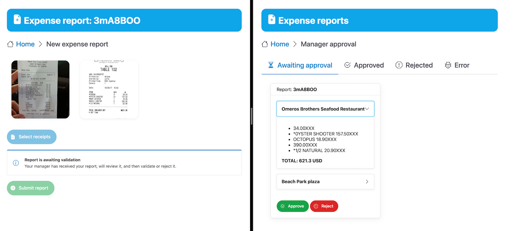
We also open sourced the code on this Github repository, if you’re interested in learning more about this application.
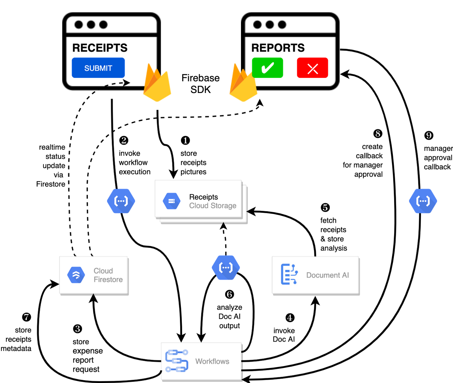
In the above diagram, there are two user journeys: the employee submitting an expense report where multiple receipts are processed at once, and the manager validating or rejecting the expense report.
First, the employee goes to the website, powered by Vue.js for the frontend progressive JavaScript framework and Shoelace for the library of web components. The website is hosted via Firebase Hosting. The frontend invokes an HTTP function that triggers the execution of our business workflow, defined using the Workflows YAML syntax.
Workflows is able to handle long-running operations without any additional code required, in our case we are asynchronously processing a set receipt files. Here, the Document AI connector directly calls the batch processing endpoint for service. This API returns a long-running operation: if you poll the API, the operation state will be “RUNNING” until it has reached a “SUCCEEDED” or “FAILED” state. You would have to wait for its completion. However, Workflows’ connectors handle such long-running operations, without you having to poll the API multiple times till the state changes. Here’s how we call the batch processing operation of the Document AI connector:
- invoke_document_ai:call: googleapis.documentai.v1.projects.locations.processors.batchProcessargs:name: ${"projects/" + project + "/locations/eu/processors/" + processorId}location: "eu"body:inputDocuments:gcsPrefix:gcsUriPrefix: ${bucket_input + report_id}documentOutputConfig:gcsOutputConfig:gcsUri: ${bucket_output + report_id}skipHumanReview: trueresult: document_ai_response
Machine learning uses state of the art Vision and Natural Language Processing models to intelligently extract schematized data from documents with Document AI. As a developer, you don’t have to figure out how to fine tune or reframe the receipt pictures, or how to find the relevant field and information in the receipt. It’s Document AI’s job to help you here: it will return a JSON document whose fields are: line_item, currency, supplier_name, total_amount, etc. Document AI is capable of understanding standardized papers and forms, including invoices, lending documents, pay slips, driver licenses, and more.
A cloud function retrieves all the relevant fields of the receipts, and makes its own tallies, before submitting the expense report for approval to the manager. Another useful feature of Workflows is put to good use: Callbacks, that we introduced last year. In the workflow definition we create a callback endpoint, and the workflow execution will wait for the callback to be called to continue its flow, thanks to those two instructions:
- create_callback:call: events.create_callback_endpointargs:http_callback_method: "POST"result: callback_details...- await_callback:try:call: events.await_callbackargs:callback: ${callback_details}timeout: 3600result: callback_requestexcept:as: esteps:- update_status_to_error:...
In this example application, we combined the intelligent capabilities of Document AI to transform complex image documents into usable structured data, with Cloud Functions for data transformation, process triggering, and callback handling logic, and Workflows enabled us to orchestrate the underlying business process and its service call logic.
Going further
If you’re looking to make sense of your documents, turning dark data into structured information, be sure to check out what Document AI offers. You can also get your hands on a codelab to get started quickly, in which you’ll get a chance at processing handwritten forms. If you want to explore Workflows, quickstarts are available to guide you through your first steps, and likewise, another codelab explores the basics of Workflows. As mentioned earlier, for a concrete example, the source code of our smart expense application is available on Github. Don’t hesitate to reach out to us at @glaforge and @asrivas_dev to discuss smart scalable apps with us.
5 Best Practices for Cloud Cost Optimization

5790
Of your peers have already read this article.
3:30 Minutes
The most insightful time you'll spend today!
When customers migrate to Google Cloud Platform (GCP), their first step is often to adopt Compute Engine, which makes it easy to procure and set up virtual machines (VMs) in the cloud that provide large amounts of computing power. Launched in 2012, Compute Engine offers multiple machine types, many innovative features, and is available in 20 regions and 61 zones!
Compute Engine’s predefined and custom machine types make it easy to choose VMs closest to your on-premises infrastructure, accelerating the workload migration process cost effectively. Cloud allows you the pricing advantage of ‘pay as you go’ and also provides significant savings as you use more compute with Sustained Use Discounts.
As Technical Account Managers, we work with large enterprise customers to analyze their monthly spend and recommend optimization opportunities. In this blog, we will share the top recommendations that we’ve developed based on our collective experience working with GCP customers.
Getting ready to save
Before you get started, be sure to familiarize yourself with the VM instance pricing page—required reading for anyone who needs to understand the Compute Engine billing model and resource-based pricing. In addition to those topics, you’ll also find information about the various Compute Engine machine types, committed use discounts and how to view your usage, among other things.
Another important step to gain visibility into your Compute Engine cost is using Billing reports in the Google Cloud Console and customizing your views based on filtering and grouping by projects, labels and more. From there you can export Compute Engine usage details to BigQuery for more granular analysis. This allows you to query the datastore to understand your project’s vCPU usage trends and how many vCPUs can be reclaimed. If you have defined thresholds for the number of cores per project, usage trends can help you spot anomalies and take proactive actions. These actions could be rightsizing the VMs or reclaiming idle VMs.
Now, with these things under your belt, let’s go over the five ways you can optimize your Compute Engine resources that we believe will give you the most immediate benefit.
1. Apply Compute Engine rightsizing recommendations
Compute Engine’s rightsizing recommendations feature provides machine type recommendations that are generated automatically based on system metrics gathered by Stackdriver Monitoring over the past eight days. Use these recommendations to resize your instance’s machine type to more efficiently use the instance’s resources. It also recommends custom machine types when appropropriate. Compute Engine makes viewing, resizing and other actions easier right from the Cloud Console as shown below.
Recently, we expanded Compute Engine rightsizing capabilities from just individual instances to managed instance groups as well. Check out the documentation for more details.
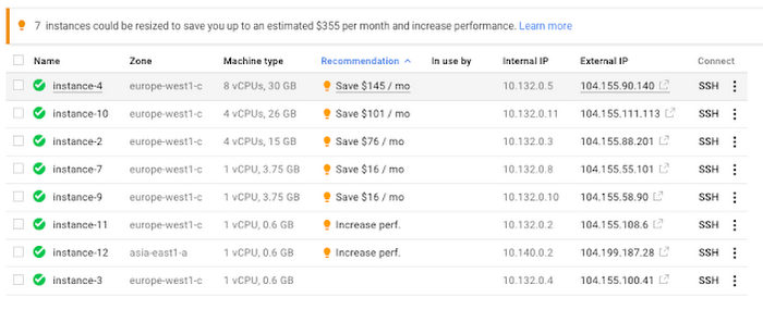
For more precise recommendations, you can install the Stackdriver Monitoring agent which collects additional disk, CPU, network, and process metrics from your VM instances to better estimate your resource requirements. You can also leverage the Recommender API for managing recommendations at scale.
2. Purchase Commitments
Our customers have diverse workloads running on Google Cloud with differing availability requirements. Many customers follow a 70/30 rule when it comes to managing their VM fleet—they have constant year-round usage of ~70%, and a seasonal burst of ~30% during holidays or special events.
If this sounds like you, you are probably provisioning resources for peak capacity. However, after migrating to Google Cloud, you can baseline your usage and take advantage of deeper discounts for Compute workloads. Committed Use Discounts are ideal if you have a predictable steady-state workload as you can purchase a one or three year commitment in exchange for a substantial discount on your VM usage.
We recently released a Committed Use Discount analysis report in the Cloud Console that helps you understand and analyze the effectiveness of the commitments you’ve purchased. In addition to this, large enterprise customers can work with their Technical Account Managers who can help manage their commitment purchases and work proactively with them to increase Committed Use Discount coverage and utilization to maximize their savings.
3. Automate cost optimizations
The best way to make sure that your team is always following cost-optimization best practices is to automate them, reducing manual intervention.
Automation is greatly simplified using a label—a key-value pair applied to various Google Cloud services. For example, you could label instances that only developers use during business hours with “env: development.” You could then use Cloud Scheduler to schedule a serverless Cloud Function to shut them down over the weekend or after business hours and then restart them when needed. Here is an architecture diagram and code samples that you can use to do this yourself.
Using Cloud Functions to automate the cleanup of other Compute Engine resources can also save you a lot of time and money. For example, customers often forget about unattached (orphaned) persistent disk, or unused IP addresses. These accrue costs, even if they are not attached to a virtual machine instance. VMs with the “deletion rule” option set to “keep disk” retain persistent disks even after the VM is deleted. That’s great if you need to save the data on that disk for a later time, but those orphaned persistent disks can add up quickly and are often forgotten! There is a Google Cloud Solutions article that describes the architecture and sample code for using Cloud Functions, Cloud Scheduler, and Stackdriver to automatically look for these orphaned disks, take a snapshot of them, and remove them. This solution can be used as a blueprint for other cost automations such as cleaning up unused IP addresses, or stopping idle VMs.
4. Use preemptible VMs
If you have workloads that are fault tolerant, like HPC, big data, media transcoding, CI/CD pipelines or stateless web applications, using preemptible VMs to batch-process them can provide massive cost savings. In fact, customer Descartes Labs reduced their analysis costs by more than 70% by using preemptible VMs to process satellite imagery and help businesses and governments predict global food supplies.
Preemptible VMs are short lived— they can only run a maximum of 24 hours, and they may be shut down before the 24 hour mark as well. A 30-second preemption notice is sent to the instance when a VM needs to be reclaimed, and you can use a shutdown script to clean up in that 30-second period. Be sure to fully review the full list of stipulations when considering preemptible VMs for your workload. All machine types are available as preemptible VMs, and you can launch one simply by adding “-preemptible” to the gcloud command line or selecting the option from the Cloud Console.
Using preemptible VMs in your architecture is a great way to scale compute at a discounted rate, but you need to be sure that the workload can handle the potential interruptions if the VM needs to be reclaimed. One way to handle this is to ensure your application is checkpointing as it processes data, i.e., that it’s writing to storage outside the VM itself, like Google Cloud Storage or a database. As an example, we have sample code for using a shutdown script to write a checkpoint file into a Cloud Storage bucket. For web applications behind a load balancer, consider using the 30-second preemption notice to drain connections to that VM so the traffic can be shifted to another VM. Some customers also choose to automate the shutdown of preemptible VMs on a rolling basis before the 24-hour period is over, to avoid having multiple VMs shut down at the same time if they were launched together.
5. Try autoscaling
Another great way to save on costs is to run only as much capacity as you need, when you need it. As we mentioned earlier, typically around 70% of capacity is needed for steady-state usage, but when you need extra capacity, it’s critical to have it available. In an on-prem environment, you need to purchase that extra capacity ahead of time. In the cloud, you can leverage autoscaling to automatically flex to increased capacity only when you need it.
Compute Engine managed instance groups are what give you this autoscaling capability in Google Cloud. You can scale up gracefully to handle an increase in traffic, and then automatically scale down again when the need for instances is lowered (downscaling). You can scale based on CPU utilization, HTTP load balancing capacity, or Stackdriver Monitoring metrics. This gives you the flexibility to scale based on what matters most to your application.
High costs do not compute
As we’ve shown above, there are many ways to optimize your Compute Engine costs. Monitoring your environment and understanding your usage patterns is key to understanding the best options to start with, taking the time to model your baseline costs up front. Then, there are a wide variety of strategies to implement depending on your workload and current operating model.
For more on cost management, check out our cost management video playlist. And for more tips and tricks on saving money on other GCP services, check out our blog posts on Cloud Storage, Networking and BigQuery cost optimization strategies. We have additional blog posts coming soon, so stay tuned!
More Relevant Stories for Your Company

How Data Teams in EdTech Firms Make Most of the Educational Data at All Levels
Education data can inform strategy, enhance both teaching and learning, and help us better understand customer needs. But that data is only as useful as an organization’s ability to access, analyze, and act upon it. Education Technology (EdTech) companies with a strong data warehouse management policy can help to make

New Enterprise Capabilities and Changes to Cloud Spanner Reduces Cost of Running Workloads by 90 Percent
Customers love Cloud Spanner because it gives them the benefits of relational semantics and SQL while also delivering the scale and availability of non-relational databases. Many of these customers want to move even more of their work to Spanner, and have requested smaller instance sizes to support development, testing and


Can Your Data Warehouse Handle a 100-Trillion Row Query?
Today's enterprise demands from data go far beyond the capabilities of traditional data warehousing and for many leaders, the need to digitally transform their businesses is a key driver for data analytics spending. Businesses want to make real-time decisions from fresh information as well as make future predictions from their

Using Google Cloud’s Backup and DR Service with Logging and Monitoring Tools
Backup and DR data is a valuable business asset, and ensuring that it’s safe and accessible is essential. In particular, you want to be able to monitor your backups to ensure that the data is indeed protected and that you can quickly recover it in the event of a disaster,
