





3079
Of your peers have already watched this video.
14:30 Minutes
The most insightful time you'll spend today!
Overview of AI Notebooks on Google Cloud
Artificial intelligence and machine learning are one of the most disruptive technologies that enterprises have encountered in the last four or five years. And AI and ML will continue to disrupt enterprises going forward for the next 10 years.
The key to unlocking value with artificial intelligence starts with a model. And the simplest way to develop a model is to use notebooks, and within notebooks to use open source frameworks to develop AI models.
Notebooks are the go-to tool for data scientists to develop and deploy AI/ML models. In this overview video, Suds Narasimhan, Product Manager, Google Cloud, walks you through an overview of cloud AI notebooks, Google Cloud’s managed Jupyter lab notebook service for enterprises on the Google Cloud.
He explores how cloud AI notebooks can help enterprise data scientists explore data quickly and develop an AI and ML model and deploy it into production.
Two Ad Agencies Leverage BigQuery to Support Next-gen Ad Campaigns

4817
Of your peers have already read this article.
2:30 Minutes
The most insightful time you'll spend today!
Advertising agencies are faced with the challenge of providing the precision data that marketers require to make better decisions at a time when customers’ digital footprints are rapidly changing. They need to transform customer information and real-time data into actionable insights to inform clients what to execute to ensure the highest campaign performance.
In this post, we’ll explore how two of our advertising agency customers are turning to Google BigQuery to innovate, succeed, and meet the next generation of digital advertising head on.
Net Conversion eliminated legacy toil to reach new heights
Paid marketing and comprehensive analytics agency Net Conversion has made a name for itself with its relentless attitude and data-driven mindset. But like many agencies, Net Conversion felt limited by traditional data management and reporting practices.
A few years ago, Net Conversion was still using legacy data servers to mine and process data across the organization, and analysts relied heavily on Microsoft Excel spreadsheets to generate reports. The process was lengthy, fragmented, and slow—especially when spreadsheets exceeded the million-row limit.
To transform, Net Conversion built Conversionomics, a serverless platform that leverages BigQuery, Google Cloud’s enterprise data warehouse, to centralize all of its data and handle all of its data transformation and ETL processes. BigQuery was selected for its serverless architecture, high scalability, and integration with tools that analysts were already using daily, such as Google Ads, Google Analytics, and Data Hub. After moving to BigQuery, Net Conversion discovered surprising benefits that streamlined reporting processes beyond initial expectations. For instance, many analysts had started using Google Sheets for reports, and BigQuery’s native integration with Connected Sheets gave them the power to analyze billions of rows of data and generate visualizations right where they were already working.If you’re still sending Excel files that are larger than 1MB, you should explore Google Cloud.
Kenneth Eisinger
Manager of Paid Media Analytics at Net Conversion
Since modernizing their data analytics stack, Net Conversion has saved countless hours of time that can now be spent on taking insights to the next level. Plus, BigQuery’s advanced data analytics capabilities and robust integrations have opened up new roads to offer more dynamic insights that help clients better understand their audience.
For instance, Net Conversion recently helped a large grocery retailer launch a more targeted campaign that significantly increased downloads of their mobile application. The agency was able to better understand and predict their customers’ needs by analyzing buyer behavior across the website, mobile application, and their purchase history. Net Conversion analyzed website data in real-time with BigQuery, ran analytics on their mobile app data through the Firebase’s integration with BigQuery, and enriched these insights with sales information from the grocery retailer’s CRM to generate propensity behavior models that accurately predicted which customers would most likely install their mobile app.
WITHIN helped companies weather the COVID storm
WITHIN is a performance branding company, focused on helping brands maximize growth by fusing marketing and business goals together in a single funnel. During the COVID-19 health crisis, WITHIN became an innovator in the ad agency world by sharing real-time trends and insights with customers through its Marketing Pulse Dashboard. This dashboard was part of the company’s path to adopting BigQuery for data analytics transformation.
Prior to using BigQuery, WITHIN used a PostgreSQL database to house its data and manual reporting. Not only was the team responsible for managing and maintaining the server, which took focus away from the data analytics, but query latency issues often slowed them down.
BigQuery’s serverless architecture, blazing-fast compute, and rich ecosystem of integrations with other Google Cloud and partner solutions made it possible to rapidly query, automate reporting, and completely get rid of CSV files.
Using BigQuery, WITHIN is able to run Customer Lifetime Value (LTV) analytics and quickly share the insights with their clients in a collaborative Google Sheet. In order to improve the effectiveness of their campaigns across their marketing channels, WITHIN further segments the data into high and low LTV cohorts and shares the predictive insights with their clients for in-platform optimizations.
By distilling these types of LTV insights from BigQuery, WITHIN has been able to use those to empower their campaigns on Google Ads with a few notable success stories.
- WITHIN worked with a pet food company to analyze historical transactional data to model predicted LTV of new customers. They found significant differences between product category and autoship vs single order customers, and they implemented LTV-based optimization. As a result, they saw a 400% increase in average customer LTV.
- WITHIN helped a coffee brand increase their customer base by 560%, with the projected 12-month LTV of newly acquired customers jumping a staggering 1280%.
Through integration with Google AI Platform Notebooks, BigQuery also advanced WITHIN’s ability to use machine learning (ML) models. Today, the team can build and deploy models to predict dedicated campaign impact across channels without moving the data. The integration of clients’ LTV data through Google Ads has also impacted how WITHIN structures their clients’ accounts and how they make performance optimization decisions.
Now, WITHIN can capitalize on the entire data lifecycle: ingesting data from multiple sources into BigQuery, running data analytics, and empowering people with data by automatically visualizing data right in Google Data Studio or Google Sheets.A year ago, we delivered client reporting once a week. Now, it’s daily. Customers can view real-time campaign performance in Data Studio — all they have to do is refresh.
Evan Vaughan
Head of Data Science at WITHIN
Having a consistent nomenclature and being able to stitch together a unified code name has allowed WITHIN to scale their analytics. Today, WITHIN is able to create an internal Media Mix Modeling (MMM) tool with the help of Google Cloud that they’re trialing with their clients.
The overall unseen benefit of BigQuery was that it put WITHIN in a position to remain nimble and spot trends before other agencies when COVID-19 hit. This aggregated view of data allowed WITHIN to provide unique insights to serve their customers better and advise them on rapidly evolving conditions.
Ready to modernize your data analytics? Learn more about how Google BigQuery unlocks the insights hidden in your data.
10189
Of your peers have already watched this video.
1:00 Minutes
The most insightful time you'll spend today!
Predict User Churn on Gaming Apps with Google Analytics Data using BigQuery ML
User retention can be a major challenge for mobile game developers. According to the Mobile Gaming Industry Analysis in 2019, most mobile games only see a 25% retention rate for users after the first day. To retain a larger percentage of users after their first use of an app, developers can take steps to motivate and incentivize certain users to return. But to do so, developers need to identify the propensity of any specific user returning after the first 24 hours.
In this blog post, we will discuss how you can use BigQuery ML to run propensity models on Google Analytics 4 data from your gaming app to determine the likelihood of specific users returning to your app.
You can also use the same end-to-end solution approach in other types of apps using Google Analytics for Firebase as well as apps and websites using Google Analytics 4. To try out the steps in this blogpost or to implement the solution for your own data, you can use this Jupyter Notebook.
Using this blog post and the accompanying Jupyter Notebook, you’ll learn how to:
- Explore the BigQuery export dataset for Google Analytics 4
- Prepare the training data using demographic and behavioural attributes
- Train propensity models using BigQuery ML
- Evaluate BigQuery ML models
- Make predictions using the BigQuery ML models
- Implement model insights in practical implementations
Google Analytics 4 (GA4) properties unify app and website measurement on a single platform and are now default in Google Analytics. Any business that wants to measure their website, app, or both, can use GA4 for a more complete view of how customers engage with their business. With the launch of Google Analytics 4, BigQuery export of Google Analytics data is now available to all users. If you are already using a Google Analytics 4 property, you can follow this guide to set up exporting your GA data to BigQuery.
Once you have set up the BigQuery export, you can explore the data in BigQuery. Google Analytics 4 uses an event-based measurement model. Each row in the data is an event with additional parameters and properties. The Schema for BigQuery Export can help you to understand the structure of the data.
In this blogpost, we use the public sample export data from an actual mobile game app called “Flood It!” (Android, iOS) to build a churn prediction model. But you can use data from your own app or website.
Here’s what the data looks like. Each row in the dataset is a unique event, which can contain nested fields for event parameters.
SELECT *FROM `firebase-public-project.analytics_153293282.events_*`TABLESAMPLE SYSTEM (1 PERCENT)
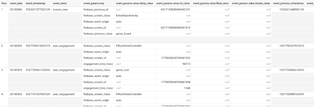
This dataset contains 5.7M events from over 15k users.
SELECTCOUNT(DISTINCT user_pseudo_id) as count_distinct_users,COUNT(event_timestamp) as count_eventsFROM`firebase-public-project.analytics_153293282.events_*
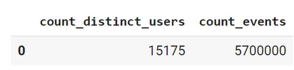
Our goal is to use BigQuery ML on the sample app dataset to predict propensity to user churn or not churn based on users’ demographics and activities within the first 24 hours of app installation.
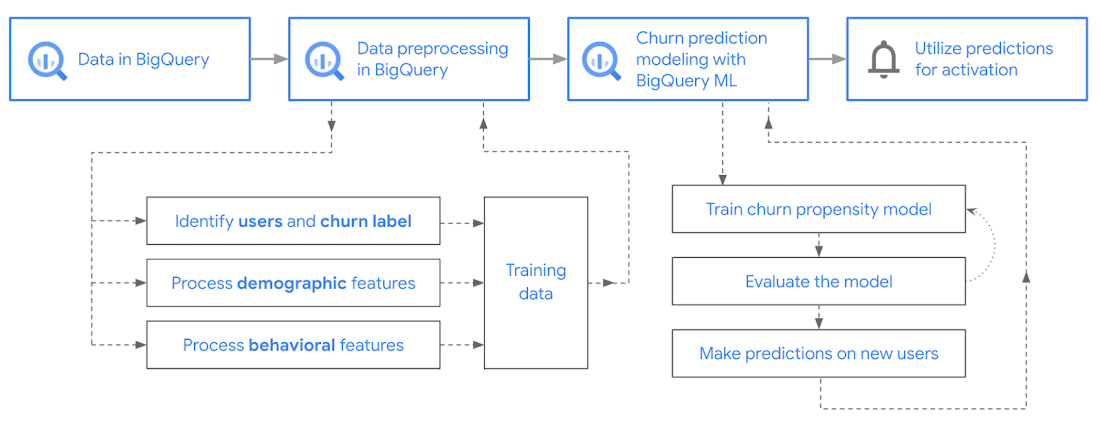
In the following sections, we’ll cover how to:
- Pre-process the raw event data from GA4
- Identify users & the label feature
- Process demographic features
- Process behavioral features
- Train classification model using BigQuery ML
- Evaluate the model using BigQueryML
- Make predictions using BigQuery ML
- Utilize predictions for activation
Pre-process the raw event data
You cannot simply use raw event data to train a machine learning model as it would not be in the right shape and format to use as training data. So in this section, we’ll go through how to pre-process the raw data into an appropriate format to use as training data for classification models.
This is what the training data should look like for our use case at the end of this section:
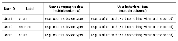
Notice that in this training data, each row represents a unique user with a distinct user ID (user_pseudo_id).
Identify users & the label feature
We first filtered the dataset to remove users who were unlikely to return the app anyway. We defined these ‘bounced’ users as ones who spent less than 10 mins with the app. Then we labeled all remaining users:
- churned: No event data for the user after 24 hours of first engaging with the app.
- returned: The user has at least one event record after 24 hours of first engaging with the app.
For your use case, you can have a different definition of bounce and churning. Also you can even try to predict something else other than churning, e.g.:
- whether a user is likely to spend money on in-game currency
- likelihood of completing n-number of game levels
- likelihood of spending n amount of time in-game etc.
In such cases, label each record accordingly so that whatever you are trying to predict can be identified from the label column.
From our dataset, we found that ~41% users (5,557) bounced. However, from the remaining users (8,031), ~23% (1,883) churned after 24 hours:
SELECTbounced,churned,COUNT(churned) as count_usersFROMbqmlga4.returningusersGROUP BY 1,2ORDER BY bounced
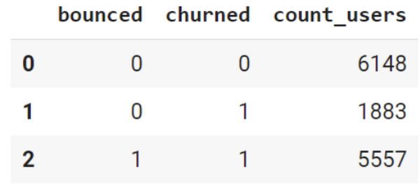
To create these bounced and churned columns, we used the following snippet of SQL code.
...#churned = 1 if last_touch within 24 hr of app installation, else 0IF (user_last_engagement < TIMESTAMP_ADD(user_first_engagement,INTERVAL 24 HOUR),1,0 ) AS churned,#bounced = 1 if last_touch within 10 min, else 0IF (user_last_engagement <= TIMESTAMP_ADD(user_first_engagement,INTERVAL 10 MINUTE),1,0 ) AS bounced,...
You can view the Jupyter Notebook for the full query used for materializing the bounced and churned labels.
Process demographic features
Next, we added features both for demographic data and for behavioral data spanning across multiple columns. Having a combination of both demographic data and behavioral data helps to create a more predictive model.
We used the following fields for each user as demographic features:
geo.countrydevice.operating_systemdevice.language
A user might have multiple unique values in these fields — for example if a user uses the app from two different devices. To simplify, we used the values from the very first user engagement event.
CREATE OR REPLACE VIEW bqmlga4.user_demographics AS (WITH first_values AS (SELECTuser_pseudo_id,geo.country as country,device.operating_system as operating_system,device.language as language,ROW_NUMBER() OVER (PARTITION BY user_pseudo_id ORDER BY event_timestamp DESC) AS row_numFROM `firebase-public-project.analytics_153293282.events_*`WHERE event_name="user_engagement")SELECT * EXCEPT (row_num)FROM first_valuesWHERE row_num = 1 #first engagement);
Process behavioral features
There is additional demographic information present in the GA4 export dataset, e.g. app_info, device, event_params, geo etc. You may also send demographic information to Google Analytics through each hit via user_properties. Furthermore, if you have first-party data on your own system, you can join that with the GA4 export data based on user_ids.
To extract user behavior from the data, we looked into the user’s activities within the first 24 hours of first user engagement. In addition to the events automatically collected by Google Analytics, there are also the recommended events for games that can be explored to analyze user behavior. For our use case, to predict user churn, we counted the number of times the follow events were collected for a user within 24 hours of first user engagement:
user_engagementlevel_start_quickplaylevel_end_quickplaylevel_complete_quickplaylevel_reset_quickplaypost_scorespend_virtual_currencyad_rewardchallenge_a_friendcompleted_5_levelsuse_extra_steps
The following query shows how these features were calculated:
WITHevents_first24hr AS (SELECTe.*FROM`firebase-public-project.analytics_153293282.events_*` eJOINbqmlga4.returningusers rONe.user_pseudo_id = r.user_pseudo_idWHERETIMESTAMP_MICROS(e.event_timestamp) <= r.ts_24hr_after_first_engagement)SELECTuser_pseudo_id,SUM(IF(event_name = 'user_engagement', 1, 0)) AS cnt_user_engagement,# ... repeated for all behavior data ...SUM(IF(event_name = 'use_extra_steps', 1, 0)) AS cnt_use_extra_steps,FROMevents_first24hrGROUP BY1
View the notebook for the query used to aggregate and extract the behavioral data. You can use different sets of events for your use case. To view the complete list of events, use the following query:
SELECTevent_name,COUNT(event_name) as event_countFROM`firebase-public-project.analytics_153293282.events_*`GROUP BY 1ORDER BYevent_count DESC
After this we combined the features to ensure our training dataset reflects the intended structure. We had the following columns in our table:
- User ID:
user_pseudo_id
- Label:
churned
- Demographic features
countrydevice_osdevice_language
- Behavioral features
cnt_user_engagementcnt_level_start_quickplaycnt_level_end_quickplaycnt_level_complete_quickplaycnt_level_reset_quickplaycnt_post_scorecnt_spend_virtual_currencycnt_ad_rewardcnt_challenge_a_friendcnt_completed_5_levelscnt_use_extra_stepsuser_first_engagement
At this point, the dataset was ready to train the classification machine learning model in BigQuery ML. Once trained, the model will output a propensity score between churn (churned=1) or return (churned=0) indicating the probability of a user churning based on the training data.
Train classification model
When using the CREATE MODEL statement, BigQuery ML automatically splits the data between training and test. Thus the model can be evaluated immediately after training (see the documentation for more information).
For the ML model, we can choose among the following classification algorithms where each type has its own pros and cons:
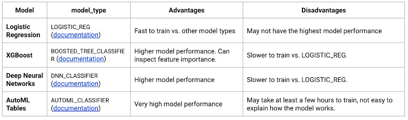
Often logistic regression is used as a starting point because it is the fastest to train. The query below shows how we trained the logistic regression classification models in BigQuery ML.
CREATE OR REPLACE MODEL bqmlga4.churn_logregTRANSFORM(EXTRACT(MONTH from user_first_engagement) as month,EXTRACT(DAYOFYEAR from user_first_engagement) as julianday,EXTRACT(DAYOFWEEK from user_first_engagement) as dayofweek,EXTRACT(HOUR from user_first_engagement) as hour,* EXCEPT(user_first_engagement, user_pseudo_id))OPTIONS(MODEL_TYPE="LOGISTIC_REG",INPUT_LABEL_COLS=["churned"]) ASSELECT*FROMbqmlga4.train
We extracted month, julianday, and dayofweek from datetimes/timestamps as one simple example of additional feature preprocessing before training. Using TRANSFORM() in your CREATE MODEL query allows the model to remember the extracted values. Thus, when making predictions using the model later on, these values won’t have to be extracted again. View the notebook for the example queries to train other types of models (XGBoost, deep neural network, AutoML Tables).
Evaluate model
Once the model finished training, we ran ML.EVALUATE to generate precision, recall, accuracy and f1_score for the model:
SELECT*FROMML.EVALUATE(MODEL bqmlga4.churn_logreg)

The optional THRESHOLD parameter can be used to modify the default classification threshold of 0.5. For more information on these metrics, you can read through the definitions on precision and recall, accuracy, f1-score, log_loss and roc_auc. Comparing the resulting evaluation metrics can help to decide among multiple models.Furthermore, we used a confusion matrix to inspect how well the model predicted the labels, compared to the actual labels. The confusion matrix is created using the default threshold of 0.5, which you may want to adjust to optimize for recall, precision, or a balance (more information here).
SELECTexpected_label,_0 AS predicted_0,_1 AS predicted_1FROMML.CONFUSION_MATRIX(MODEL bqmlga4.churn_logreg)
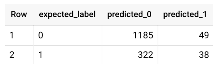
This table can be interpreted in the following way:

Make predictions using BigQuery ML
Once the ideal model was available, we ran ML.PREDICT to make predictions. For propensity modeling, the most important output is the probability of a behavior occurring. The following query returns the probability that the user will return after 24 hrs. The higher the probability and closer it is to 1, the more likely the user is predicted to return, and the closer it is to 0, the more likely the user is predicted to churn.
SELECTuser_pseudo_id,returned,predicted_returned,predicted_returned_probs[OFFSET(0)].prob as probability_returnedFROMML.PREDICT(MODEL bqmlga4.churn_logreg,(SELECT * FROM bqmlga4.train)) #can be replaced with a proper test dataset
Utilize predictions for activation
Once the model predictions are available for your users, you can activate this insight in different ways. In our analysis, we used user_pseudo_id as the user identifier. However, ideally, your app should send back the user_id from your app to Google Analytics. In addition to using first-party data for model predictions, this will also let you join back the predictions from the model into your own data.
- You can import the model predictions back into Google Analytics as a user attribute. This can be done using the Data Import feature for Google Analytics 4. Based on the prediction values you can Create and edit audiences and also do Audience targeting. For example, an audience can be users with prediction probability between 0.4 and 0.7, to represent users who are predicted to be “on the fence” between churning and returning.
- For Firebase Apps, you can use the Import segments feature. You can tailor user experience by targeting your identified users through Firebase services such as Remote Config, Cloud Messaging, and In-App Messaging. This will involve importing the segment data from BigQuery into Firebase. After that you can send notifications to the users, configure the app for them, or follow the user journeys across devices.
- Run targeted marketing campaigns via CRMs like Salesforce, e.g. send out reminder emails.
You can find all of the code used in this blogpost in the Github repository:
What’s next?
Continuous model evaluation and re-training
As you collect more data from your users, you may want to regularly evaluate your model on fresh data and re-train the model if you notice that the model quality is decaying.
Continuous evaluation—the process of ensuring a production machine learning model is still performing well on new data—is an essential part in any ML workflow. Performing continuous evaluation can help you catch model drift, a phenomenon that occurs when the data used to train your model no longer reflects the current environment.
To learn more about how to do continuous model evaluation and re-train models, you can read the blogpost: Continuous model evaluation with BigQuery ML, Stored Procedures, and Cloud Scheduler
More resources
If you’d like to learn more about any of the topics covered in this post, check out these resources:
- BigQuery export of Google Analytics data
- BigQuery ML quickstart
- Events automatically collected by Google Analytics 4
- Qwiklabs: Create ML models with BigQuery ML
Or learn more about how you can use BigQuery ML to easily build other machine learning solutions:
- How to build demand forecasting models with BigQuery ML
- How to build a recommendation system on e-commerce data using BigQuery ML
Let us know what you thought of this post, and if you have topics you’d like to see covered in the future! You can find us on Twitter at @polonglin and @_mkazi_.Thanks to reviewers: Abhishek Kashyap, Breen Baker, David Sabater Dinter.
6192
Of your peers have already watched this video.
18:00 Minutes
The most insightful time you'll spend today!
An Overview of Google’s Data Cloud
Data access, management and privacy has been at the center of priorities for enterprises that are aiming to be more agile, reliable and data-driven. Google Cloud’s technology innovations spanning products like BigQuery, Spanner, Looker and VertexAI help organizations navigate the complexities related to siloed data in large volumes sprawled across databases, data lakes, data warehouses, and data marts in multiple clouds and on-premises. Watch the video to learn how companies are building data on Google Cloud for better analysis, security and management to achieve bottomline!
Experts’ Guideline for Personalizing Platforms with the Right Recommendation System on Google Cloud

5019
Of your peers have already read this article.
5:00 Minutes
The most insightful time you'll spend today!
Over the past two decades, consumers have become accustomed to receiving personalized recommendations in all facets of their online life. Whether that be recommended products while shopping on Amazon, a curated list of apps in the Google Play store, or relevant videos to watch next on YouTube. In fact, in a Verge article “How YouTube perfected the feed: Google Brain gave YouTube new life,” the Google Brain team reveals how their recommendation engine has impacted the platform with “more than 70 percent of the time people spend watching videos on the site being driven by YouTube’s algorithmic recommendations” thereby increasing time spent on the platform by 20X in three years.
It’s become clear that personalized recommendations are no longer a differentiator for an organization but rather something consumers have come to expect in their day-to-day experiences online. So what should you do if you are behind the curve and want to get started or simply want to improve upon what you already have? While there are all sorts of techniques, from content-based systems to deep learning methods, our goal in this recommender-focused blog series is to demystify three available approaches to building recommendation systems on Google Cloud: Matrix Factorization in BigQuery Machine Learning (BQML), Recommendations AI, and deep retrieval techniques available via the Two-Tower built-in algorithm.
One of these approaches can be used to meet you where you are in your personalization journey, no matter if you are just starting or if you are well into it. This first blog post will introduce our three approaches and when to use them.
What is Matrix Factorization and how does it work?
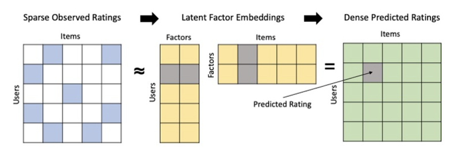
Collaborative filtering is a foundational model for building a recommendation system as the input dataset is simple and the embeddings are learned for you. How does Matrix factorization fit into the mix you might be wondering? Matrix factorization is simply the model that applies collaborative filtering. BQML enables users to create and execute a matrix factorization model by using standard SQL directly in the data warehouse.
Collaborative filtering begins by creating an interaction matrix. The interaction matrix represents users as a row and items as columns in your dataset. This interaction matrix often is sparse in nature as not all users will have interacted with many items in your catalog. This is where embeddings come into play. Generating embeddings for users and items not only allows you to collapse many sparse features into a lower dimensional space but they also allow you to derive a similarity measure so that similar users/items fall nearby in the embedding space. These similarity measures are key as collaborative filtering uses similarities between users and items to make the end recommendations. The underlying assumption being that similar users will like similar items whether that be movies or handbags.
What’s required to get started?
To train a matrix factorization model you need a table that includes three input columns: user(s), item(s), and an implicit or explicit feedback variable (e.g., ratings is an example of explicit feedback). With the base input dataset in place, you can then easily run your model in BigQuery after specifying several hyperparameters in your CREATE MODEL SQL statement. Hyperparameters are available to specify the number of embeddings, the feedback type, the amount of L2 regularization applied and so on.
Why use this approach and who is it a good fit for?
As mentioned earlier, Matrix Factorization in BQML is a great way for those new to recommendation systems to get started. Matrix factorization has many benefits:
- Little ML Expertise: Leveraging SQL to build the model lowers the level of ML expertise needed
- Few Input Features: Data inputs are straightforward, requiring a simple interaction matrix
- Additional Insight: Collaborative filtering is adept at discovering new interests or products for users
While Matrix Factorization is a great tool for deriving recommendations it does come with additional considerations and potential drawbacks depending upon the use case.
- Not Amenable to Large Feature Sets: The input table can only contain two feature columns (e.g., user(s), item(s)). If there is a need to include additional features such as contextual signals, Matrix factorization may not be the right method for you.
- New Items: If an item is not available in the training data, the system can’t create an embedding for it and will have difficulty recommending similar items. While there are some workarounds available to address this cold-start issue, if your item catalog often includes new items, Matrix factorization may not be a good fit.
- Input Data Limitations: While the input matrix is expected to be sparse, training examples without feedback can cause problems. Filtering for items and users that have at least a handful of feedback (e.g., ratings) examples can improve the model. More information on limitations can be found here.
In summary, for users with a simplified dataset looking to iterate quickly and develop a baseline recommendation system, Matrix Factorization is a great approach to begin your personalization AI journey.
What is Recommendations AI and how does it work?
Recommendations AI is a fully managed service which helps organizations deploy scalable recommendation systems that use state-of-the-art deep learning techniques, including cutting-edge architectures such as two-tower encoders, to serve personalized and contextually relevant recommendations throughout the customer journey.
Deep learning models are able to improve the context and relevance of recommendations in part because they can easily address the previously mentioned limitations of Matrix Factorization. They incorporate a wide set of user and item features, and by definition they emphasize learning successive layers of increasingly meaningful representations from these features. This flexibility and expressivity allows them to capture complex relationships like short-lived fashion trends and niche user behaviors. However, this increased relevance comes at a cost, as deep learning recommenders can be difficult to train and expensive to serve at scale.
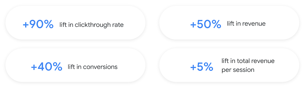
Recommendations AI helps organizations take advantage of serving these deep learning models and handles the MLOps required to serve these models globally with low latency. Models are automatically retrained daily and tuned quarterly to capture changes in customer behavior, product assortment, pricing, and promotions. Newly trained models follow a resilient CI/CD routine which validates they are fit to serve and promotes them to production without service interruption. The models achieve low serving latency by using a scalable approximate nearest neighbors (ANN) service for efficient item retrieval at inference time. And, to maintain consistency between online and offline tasks, a scalable feature store is used, preventing common production challenges such as data leakage and training-serving skew.
What’s required to get started?
To get started with Recommendations AI we first need to ingest product and user data into the API:
- Import product catalog: For large product catalog updates, ingest catalog items in bulk using the catalogItems.import method. Frequent catalog updates can be schedule with Google Merchant Center or BigQuery
- Record user events: User events track actions such as clicking on a product, adding items to cart, or even purchasing an item. These events need to be ingested in real time to reflect the latest user behavior and then joined to items imported in the product catalog
- Import historical user events: The models need sufficient training data before they can provide accurate predictions. The recommended user event data requirements are different across model types (learn more here)
Once the data requirements are met, we are able to create one or multiple models to serve recommendations:
- Determine your recommendation types and placements: The location of the recommendation panel and the objective for that panel impact model training and tuning. Review the available recommendations types, optimization objectives, and other model tuning options to determine the best options for your business objectives.
- Create model(s): Initial model training and tuning can take 2-5 days depending on the number of user events and size of the product catalog
- Create serving configurations and preview recommendations: After the model is activated, create serving configurations and preview the recommendations to ensure your setup is functioning as expected before serving to production traffic
Once models are ready to serve, consider setting up A/B experiments to understand how newly trained models impact your customer experience before serving them to 100% of your traffic. In the Recommendations AI console, see the Monitoring & Analytics page for summary and placement-specific metrics (e.g., recommender-engaged revenue, click-through-rate, conversion rate, and more).
Why use this approach and who is it a good fit for?
Recommendations AI is a great way to engage customers and grow your online presence through personalization. It’s used by teams who lack technical experience with production recommendation systems, as well as customers who have this technical depth but want to allocate their team’s effort towards other priorities and challenges. No matter your team’s technical experience or bandwidth, you can expect several benefits with Recommendations AI:
- Fully managed service: no need to preprocess data, train or hypertune machine learning models, load balance or manually provision you infrastructure – this is all taken care of for you. The recommendation API also provides a user-friendly console to monitor performance over time.
- State-of-the-art AI: take advantage of the same modeling techniques used to serve recommendations across Google Ads, Google Search, and YouTube. These models excel in scenarios with long-tail products and cold-starts users and items
- Deliver at any touchpoint: serve high-quality recommendations to both first-time users and loyal customers anywhere in their journey via web, mobile, email, and more
- Deliver globally: serve recommendations in any language anywhere in the world at low-latency with a fully automated global serving infrastructure
- Your data, your models: Your data and models are yours. They’ll never be used for any other Google product nor shown to any other Google customer
For users looking to leverage state of the art AI to fuel their recommendation systems but need an existing solution to get up and running more quickly, Recommendations AI is the right solution for you.
What are Two Tower encoders and how do they work?
As a reminder, in recommendation system design, our objective is to surface the most relevant set of items for a given user or set of users. The items are usually referred to as the candidate(s) where we might include information about the items such as the title or description of the item, other metadata about the item like language, number of views, or even clicks on the item over time. User(s) are often represented in the form of a query to a recommendation system where we might provide details about the user such as the location of the user, preferred languages, and what they have searched for in the past.
Let’s start with a common example. Imagine that you are creating a movie recommendation system. The input candidates for such a system would be thousands of movies and the query set can consist of millions of viewers. The goal of the retrieval stage is to select a smaller subset of movies(candidates) for each user and then score and rank order them before presenting the final recommended list to the query/user.
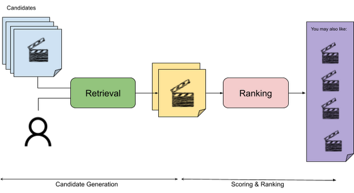
The retrieval stage is able to refine our list of candidates by encoding both the candidate and the query data so they share the same embedding space. A good embedding space will place candidates which are similar to one another closer together and dissimilar items/queries farther apart in the embedding space.
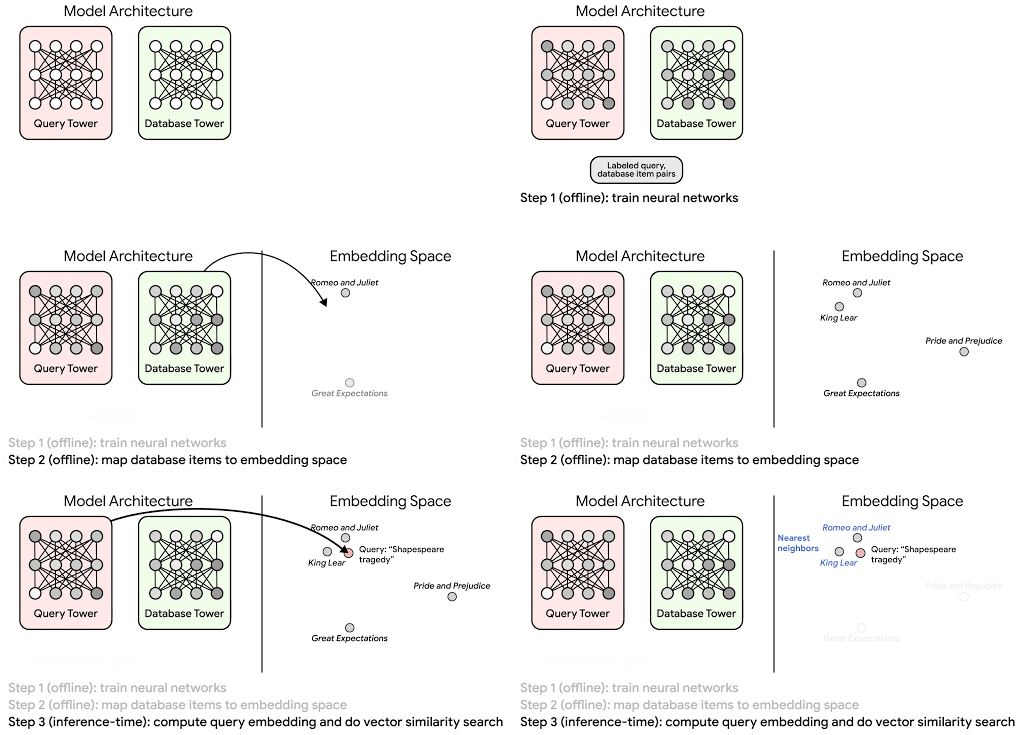
Once we have a database of query and candidate embeddings we can then use an approximate nearest neighbor search method to then generate a list of final “like” candidates, i.e. find a certain number of nearest neighbors for a given query/user and surface final recommendations.
What’s required to get started?
At the most basic level, in order to train a two-tower model you need the following inputs:
- Training Data: Training data is created by combining your query/user data with data about the candidates/items. The data must include matched pairs, cases where both user and item information is available. Data in the training set can include many formats from text, numeric data, or even images.
- Input Schema: The input schema describes the schema of the combined training data along with any specific feature configurations.
Several services within Vertex AI have come available that complement the existing Two-Tower built-in algorithm and can be leveraged in your execution:
- Nearest Neighbor (ANN) Service: Vertex AI Matching Engine and ScANN provide a high-scale and low-latency Approximate Nearest Neighbor (ANN) service so you can more easily identify similar embeddings.
- Hyperparameter Tuning Service: A hyperparameter tuning service such as Vizier can help you identify the optimal hyperparameters such as the number of hidden layers, the size of the hidden layers, and the learning rate in fewer trials.
- Hardware Accelerators: Specialized hardware, such as GPUs or TPUs, can be valuable in your recommendation system to help accelerate experiments and improve the speed of training cycles.
Why use this approach and who is it a good fit for?
The Two-Tower built-in algorithm can be considered the “custom sports car” of recommendation systems and comes with several benefits:
- Greater Control: While Recommendations AI uses the two-tower architecture as one of the available architectures it doesn’t provide granular control or visibility into model training, example generation, and model validation details. In comparison, the Two-Tower built in algorithm provides a more customizable approach as you are training a model directly in a notebook environment.
- More Feature Options: The Two Tower approach can handle additional contextual signals ranging from text to images.
- Cold Start Cases: Leveraging a rich set of features not only enhances performance but also allows the candidate generation to work for new users or new candidates.
While the Two-Tower built in algorithm is an excellent and best-in class solution for deriving recommendations, it does come with additional considerations and potential drawbacks depending upon the use case.
- Technical ML Expertise Required: Two tower encoders are not a “plug and play” solution like the other approaches mentioned above. In order to effectively leverage this approach, appropriate coding and ML expertise is required.
- Speed to Insight: Building out a custom solution via two-tower encoders may require additional time as the solution is not pre-built for the user.
For users looking for greater control, increased flexibility, and have the technical chops to easily work within a managed notebook environment – the two-tower built in algorithm is the right solution for them.
What’s next?
In this article, we explored three common methods for building recommendation systems on Google Cloud Platform. As you can see thus far, there are alot of considerations to take into account before choosing a final approach. In an effort to help you align more quickly we have distilled the decision criteria down to a few simple steps (see below for more details).
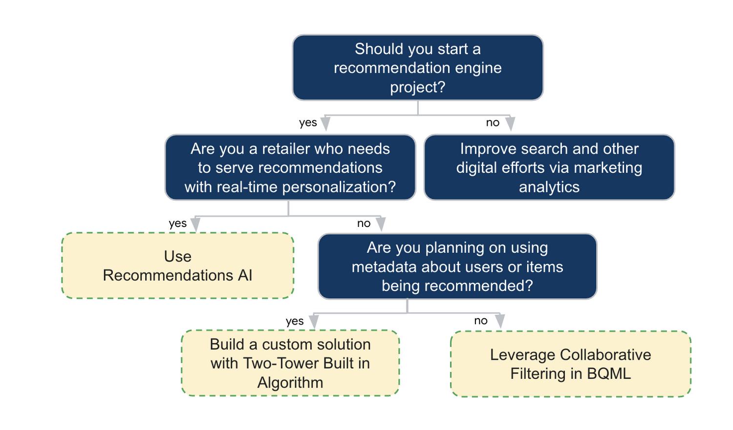
In the next installments of this series, we will dive more deeply into each method, explore how hardware accelerators can play a key role in recommendation system design, and discuss how recommendation systems may be leveraged in key verticals. Stay tuned for future posts in our recommendation systems series. Thank you for reading! Have a question or want to chat? Find authors here – R.E. [Twitter | LinkedIn], Jordan [LinkedIn], and Vaibhav [LinkedIn].
Acknowledgements
Special thanks to Pallav Mehta, Henry Tappen,Abhinav Khushraj, and Nicholas Edelman for helping to review this post.
References
UKG Ready: Meeting the Needs of Complex Machine Learning Models and Distributed Data Sets

3987
Of your peers have already read this article.
2:30 Minutes
The most insightful time you'll spend today!
Business Problem
UKG Ready primarily operates in the Small and Medium Business (SMB) space, so inherently many customers are forced to operate and make key business decisions with less Workforce Management (WFM) / Human Capital Management (HCM) data. In addition to volume, SMB lacks the variety of data needed to create a dynamic and agile organization. This puts SMB at a major disadvantage compared to larger segments.
Project Goals
People Insights module is committed to surfacing insights to customers in the context of their day-to-day duties and aid in decision making. With the SMB customer data limitations mentioned above, the goal of this project was to create a global dataset that augments individual customer data to bring light to less obvious, yet important information.
Challenges
UKG Ready is a highly configurable application that gives customers the opportunity to build solutions on a platform that meets their specific business needs. High configurability gives high flexibility to customers in their usage of the software. However, it becomes nearly impossible to create a global dataset for machine learning and data insights. UKG Ready manages just under 4 million of the US workforce and some 30,000+ customers. Despite the large employee dataset size, machine learning models that are specific to customers are starved for data because the individual customers have a relatively small employee population. Does that mean we cannot support our SMB customers’ decision making with ML?
Result
Partnering with Google, we were able to develop an approach that allowed us to standardize various domain entities (pay categories, time off codes, job titles, etc.) so that we could build a global dataset to augment SMB customer data. Using machine learning we were able to build a common vocabulary across our customer base. This common vocabulary encapsulates the nuances of how our customers manage their business and yet is generalized and standardized such that the data can be aggregated over the variety of customer configurations. This allows us to serve up practical insights to customers through various use cases. Our partnership allowed us to leverage Google Cloud Services to meet the needs of our complex machine learning models, distributed data sets and CI/CD processes.
How
UKG Ready decided to partner with Google for an end-to-end solution for the analytics offering. This allowed us to focus on our core business logic without having to worry about the platform, environment configurations, performance and scalability of the entire solution. We make use of various Google Cloud services such as Cloud Triggers, Cloud Storage, Cloud Functions, Cloud Composer, Cloud Dataflow, Big Query, Vertex AI, Cloud Pub/Sub… to host our analytics solution. Jenkins manages the entire CI/CD pipelines and cloud environments are configured and deployed using Terraform.
The standardization of business entities problem was solved in three distinct steps:
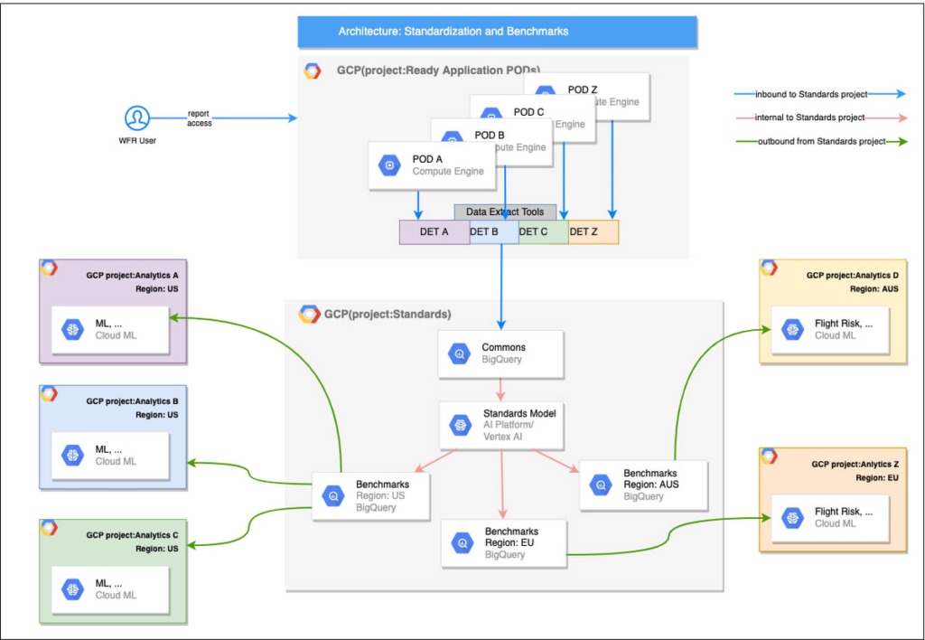
Step 1: Collecting aggregated data
We needed an approach to collect aggregated data from our highly distributed, sharded, multi-tenant data sources. We developed a custom solution that allows us to extract data aggregated at source for PII and GDPR considerations and transfer to Google Cloud Storage in the fastest manner possible. Data is then transformed and stored in Big Query. Services used: GCS, Cloud Functions, DataFlow, Cloud Composer and Big Query. All processes are orchestrated using Cloud Composer and detailed logging is available in Cloud Logging (Stackdriver).
Step 2: Applying NLP (Natural Language Processing)
Once we had the variety of customer configurations or the business entities available, we then applied NLP algorithms to categorize and standardize these in buckets. This approach assumes that customers use natural language for configurations like job titles, pay codes etc.
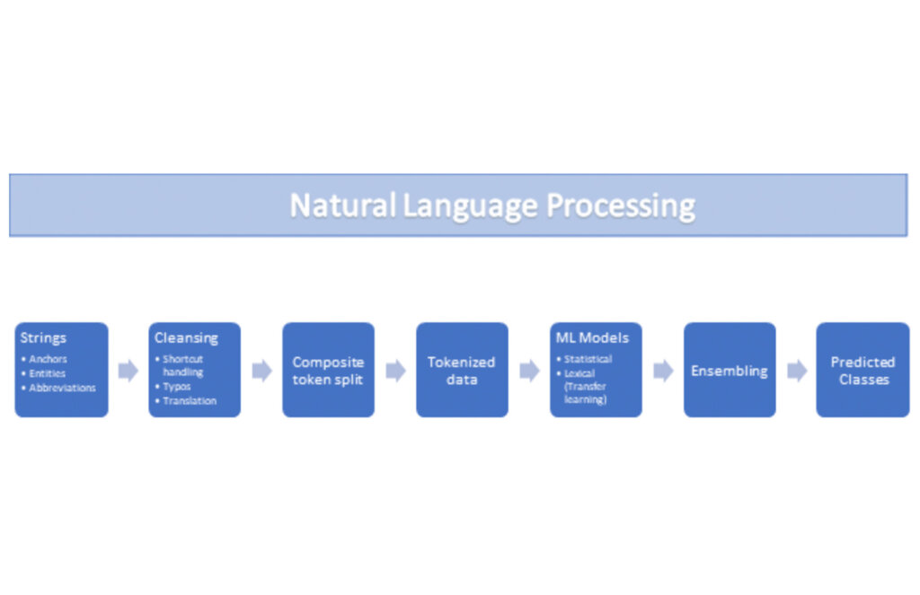
String Preparation
The input data for string preparation process is an entity string or several strings, that describe one entity object (like name-description pair or code-name pair). The output represents set of tokens that may be used to run a classification/clustering model. The process of string preparation tokenizes strings, replaces shortcuts, handles abbreviations, translates tokens, handles grammatical errors and mistypes
ML Models
Statistical
The idea of the model is to use defined target classes (clusters) and assign several tokens (anchors) to each of them an entity that has any of those tokens would be “attracted” to appropriate class. All other tokens are weighted according to frequencies of usage of theses tokens in the entities with anchor tokens:
Using anchor tokens, we are building kind-of Word2Vec - dimensionality of vector is equal to number of target classes. The higher the specific dimension (cluster) value, the higher the probability of entity to be included in appropriate cluster. Final prediction for entity tokens list for specific class is sum of weights of all the tokens included. Predicted cluster is a cluster that has maximal prediction score.
Lexical Model
We managed to generate reasonable amount of labeled data during statistical model implementation and testing. That opens a possibility to build “classical” NLP model that uses labeled data to train classification neural network using pretrained layers to produce token embeddings or even string embeddings. We started experimentation with pre-trained models like GloVe and got good results with single words and bi-grams but started getting issues in handling of n-grams. Our Google account team came to our rescue and recommended some white papers that helped formulate our strategy. We now use Tensorflow nnlm-en-dim128 model to produce string embeddings – it was trained on 200B records English Google News corpus and produces for each input string 128-dimensional vector. After that we use several Dense and Dropout layers to build a classification model.
Ensembling
To perform ensembling all the model results for each class are cast to probabilities using softmax transformation with scale normalization. Final predicted probability is maximal average score of both models among all the classes scores – appropriate class is predicted class.
The machine learning models are deployed on Vertex AI and are used in batch predictions. Model performance is captured at every prediction boundary and monitored for quality in production.
Step 3: Making available common vocabulary
Having the standardized vocabulary, we then needed a mechanism to have the results be available in UKG Ready reports and customer specific models like Flight Risk and Fatigue. For this we again used Google Services for orchestration, data transformation and data storage.
Once the modeling is complete, we made the customer specific models leveraging the above architecture be available in Reports. We utilized our proven existing technology choices in GCP for orchestration, data transformation and data storage
Results
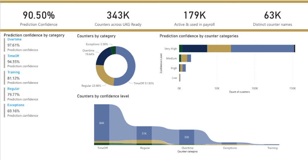
We are able to build a common vocabulary of our customers’ business entities with good confidence. And be an expert advisor to our SMB customers in their decision-making using machine learning. With the advice of our Google account team and using Google services we can add value to our product in a relatively short amount of time. And we are not done! We continue to use this platform for new use cases, complex business problems and innovative machine learning solutions.
Sample result:
Special thanks to Kanchana Patlolla , AI Specialist, Google for the collaboration in bringing this to light
More Relevant Stories for Your Company

Introducing Duet AI on Google Cloud: AI-Powered Developer Productivity Unleashed
Last week we announced the private preview of Duet AI for Google Cloud, an always-on AI collaborator that uses generative AI to provide help to developers and cloud users. This article gives you a detailed look at Duet AI for developers, showing how Duet AI can help provide developers with real-time code

Johnson & Johnson Increases it’s Ability to Find Highly Qualified Staffers for Business Critical Roles by 41% with Easy-to-Use AI
Job seekers can often feel lost or disconnected—like the right opportunity is out there, but they don’t know where or how to look. Employers face a similar challenge when trying to attract the right candidates. Many companies, especially large enterprises, face a talent shortage across a range of critical roles. For global

Everything a Marketer Needs to Know About Machine Learning
As consumer expectations grow for more personalized, relevant, and assistive experiences, machine learning is becoming an invaluable tool to help meet those demands. It’s helping marketers create smarter customer segmentations, deliver more relevant creative campaigns, and measure performance more effectively. In fact, 85% of executives believe AI will allow their

Google Cloud Next ’22 to Commence in October: Block Your Calendar!
We’re excited to announce that Google Cloud Next returns on October 11–13, 2022. Join us for keynotes from industry luminaries and engage live with Google developers. Explore dynamic content across various learning levels, and dive deep into technologies and solutions spanning the Google Cloud and Google Workspace portfolios. Participate in breakout sessions,
