





Vodafone Leverages Google Cloud to Aid COVID-19 Frontline with Anonymized Insights on Population Mobility

11175
Of your peers have already read this article.
1:30 Minutes
The most insightful time you'll spend today!
Editor’s note: When Europe’s largest mobile communications company, Vodafone, was asked by the European Commission to help understand population movement across the European Union and the UK to help fight COVID-19, it was able to provide anonymized mobile network-based insights to answer the call. Here’s how Vodafone, with the support of Google Cloud, rapidly mobilized the COVID-19 frontline, while respecting its customers’ privacy.
With the emergence of COVID-19 in early 2020, the European Commission—the executive branch of the European Union (EU)—knew that technology would be instrumental in its fight to control the pandemic. With various lockdowns imposed across its member states, the Commission was keen to predict and prevent the spread of COVID-19 and to manage the related social, political and financial impacts.
Mobile network data helps track COVID-19 across the EU
Mobile networks produce location data, which can be turned into useful anonymous insights to understand population movement within a geographic area. The European Commission, working with mobile industry association GSMA (Groupe Speciale Mobile Association), asked Europe’s major mobile phone operators for help in producing insights to support the fight against COVID-19. As the largest mobile network operator within the EU, Vodafone saw this as a critical opportunity to participate.
Vodafone had previous experience of using mobile network data to support pandemic research. For example, in 2019, Vodafone provided mobility pattern analysis to help track the spread of Malaria in Mozambique. And, during the early stages of the COVID-19 pandemic (prior to working with the European Commission), Vodafone assisted the Italian and Spanish governments in understanding their citizens’ mobility patterns. Vodafone had also previously offered anonymized and aggregated population mobility insights to support public transport and tourism authorities and retail organizations in a number of countries. Consequently, Vodafone was perfectly placed to play a greater role in supporting the European Commission’s response to the pandemic.
When asked to assist the European Commission, Vodafone first considered how it could safely share its data with the governing body without providing details on the individual movements of its customers. It realized it could achieve this through an elaborate set of anonymization and aggregation techniques. Insights are aggregated from a minimum of 50 users and Vodafone only shared these anonymous insights and never the actual raw data with the Commission. As specified by the EU, these insights are then presented onto a large geographical region, typically a city or a county with thousands of people living in that area.
These insights illustrate how people move, helping to determine how lockdowns and self-isolation measures were impacting behaviors.
Using Google Cloud to collate and store population mobility data
In April 2020, Vodafone began migrating its operations, including its mobile data, to Google Cloud on servers in Europe and the UK with elaborate security safeguards, including encryption, building on a previous partnership.
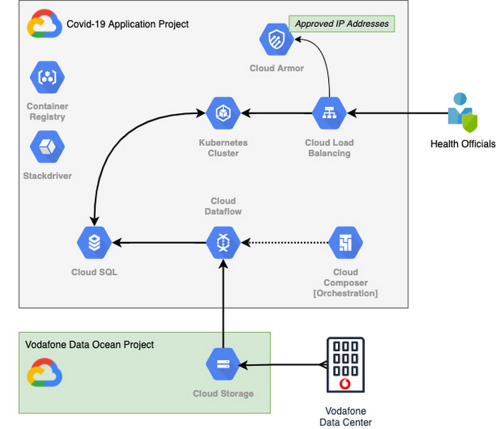
With the data residing in EU and UK data centers and not the United States, Vodafone could then retrieve anonymous insights from Google Cloud Storage instantaneously. Before supplying any information to the European Commission, however, Vodafone used Dataflow to validate the data and run a series of tests to ensure the database had accurate data, before ingesting and archiving the relevant metrics. For instant access, the data was then made available to the European Commission using a Redis database on Google Kubernetes Engine.
To ensure aggregate Vodafone customer data was always safe, secure, and anonymous, all entry points to the front-end were protected behind Google Cloud Armor, where only specific IP addresses were allowed. Using these tools, seamless data pipelines fed in predefined key performance indicators from each specified European market. While data quality measures ensured the definitions for metrics across markets were consistent and could be accurately compared.
The architecture (pictured below) shows how Vodafone integrated and anonymized its data on Google Cloud.
Live interactive dashboard shows population mobility in real-time
With its data integrated on Google Cloud, Vodafone created a live, interactive dashboard to track mobility patterns and share relevant information with the European Commission in real-time.
The European Commission Joint Research Center (JRC) was able to gather valuable information from these insights, which enabled them to see where population mobility was aiding the spread of the disease, when cross-referenced with health data. It could also assess the implications of lockdowns on different populations and forecast cross-country spreading.
Mobile data aids disease modeling for multiple stakeholders
The Vodafone data became instrumental in modeling the likely course of the disease too. For example, the University of Southampton in the UK used it to predict the outcome of different coordinated COVID-19 exit strategies across Europe. This research was published in Science Magazine in September 2020.
The Vodafone data dashboard continues to be used by individual governments, NGOs and organizations to further investigate the impacts of the pandemic and to measure the effectiveness of response strategies alongside the rollout of vaccination programs. The project also helped Vodafone win a DataIQ award for most effective stakeholder engagement.
Using the learnings from this project, Vodafone has been able to adapt its own B2B solution, called Vodafone Analytics, by adaptIng and migrating the code to work in Google Cloud Platform. This solution has been rolled out across Germany, Greece, Portugal and South Africa, and new countries are being onboarded every day. Vodafone Analytics already has more than 100 customers leveraging it for a variety of use cases—Italian fashion retailer OVS, uses it for its smart retail operation, while global real estate company, JLL, uses it to understand the footfall passing through its properties.
Working together, Vodafone and Google Cloud continue to help a range of organizations, governments, and NGOs navigate through the ongoing pandemic, optimize their operations, and help the greater good, without infringing individuals’ fundamental rights to privacy.
To learn more about Google Cloud and Vodafone, watch our full interview here.
Anthos for Manufacturing: Tackle DevOps Complexities and Drive Digital Transformation
DOWNLOAD E-BOOK6250
Of your peers have already downloaded this article
2:00 Minutes
The most insightful time you'll spend today!
Google Cloud Accelerates Financial Organizations’ Journey towards Digital Transformation

10456
Of your peers have already read this article.
2:00 Minutes
The most insightful time you'll spend today!
When I reflect back on the past year and the pandemic, I’m struck by how the reliance on remote work and operations has changed the fundamentals of business forever. For the financial services industry, this rings particularly true. Many conversations I’m having right now with organizations revolve around embracing a transformation cloud, and thinking of cloud computing not just as an infrastructure decision, but also as the locus for transformation throughout the company.
Today, as we welcome the industry to our Financial Services Summit, we’ll demonstrate just how Google Cloud accelerates a financial organization’s digital transformation through app and infrastructure modernization, data democratization, people connections, and trusted transactions. We hope you’ll join us.
How we’re helping financial services firms build their transformation clouds
At Google Cloud, we continue to focus on areas where we can bring the best of our capabilities to banking, capital markets, insurance, and payments customers around the world. Our work with financial services industry customers has given us a deep understanding of the real-world, specific use cases that matter most to them. This groundwork led us to engineer products and solutions that are open and flexible, not ones that force them to rip out existing investments in ERP or other early IaaS cloud implementations.
It’s why we’ve engineered solutions such as Lending DocAI, Open Banking with Apigee, and Datashare for financial services to help transform the industry. These solutions were created with our customers’ security and compliance top-of-mind and are built at the intersection of user-optimized experience, technology, and sovereignty.
At their core, financial institutions want to drive growth, reduce costs, mitigate risk, stay compliant, and increase efficiency. As a result, when we partner with them on their transformation journeys, we consider three essential focus areas:
- Enabling the human experience and connected interactions
- Building an open and intelligent data foundation for better insights
- Providing the most trusted and secure cloud in the industry
Enabling humans and connected interactions
A company’s transformation is about more than technology; people and culture ultimately drive change. HSBC, for example, recognized its business users would benefit from guided answers to common questions around risk policy compliance, and turned to Google Cloud to leverage AI and machine learning bots to assist employees, ease the burden on policy experts, and improve the user experience. Using Dialogflow, a core component of Contact Center AI, HSBC was able to build a conversational platform that quickly and accurately addresses user needs at scale.
Another example is Equifax, which used Google Workspace to support collaboration not only internally between employees, but also externally with customers. Customers can use Google Cloud solutions for financial services to build these sorts of technology-enabled human interactions quickly and easily—supporting organizational change at scale.
Building an open and intelligent data foundation for smarter, faster insights
The real impact of Google Cloud solutions for financial services comes when the whole company has access to the right information at the right time, and can act more intelligently on that data. Our solutions help businesses safely leverage their data and get a complete 360-degree view of their customers’ information, which can often be scattered across multiple systems (CRM, lending, credit, etc.). This helps financial institutions improve the overall customer experience—and sometimes even develop new products quickly.
Indeed, all financial institutions are looking for ways to grow revenue and reduce expenses, and data can be a critical ingredient to doing both effectively. As daily transactions rise, so does the volume and complexity of data. But to implement new customer experience innovations (and new revenue streams), financial institutions must first capture data effectively. This is why AXA Switzerland, for example, uses real-time analytics on Google Cloud to gain cross-industry insights about future trends and customer preferences.
Financial services organizations also need the confidence of building on a platform that provides choice, flexibility, and agility to move fast. It’s why we have an open cloud approach that allows Google Cloud services to run in different physical locations such as on-premises, other public clouds, and the edge. Customers can also harness the power of data and AI through our open APIs, machine-learning services, and analytics engines on any major cloud platform. This is why companies like Macquarie Bank are taking advantage of Google Cloud’s open, hybrid architecture to modernize and empower its developers.
Compliant and secure to address risk and regulatory needs
As a highly regulated industry, financial services is focused on security and compliance, risk and regulations, and fraud detection and prevention. Google Cloud offers unique capabilities to earn customers’ trust as part of our continuing work to be the most trusted cloud in the industry. Google Cloud provides a secure foundation that you can verify and independently control. Our cloud technology reduces risk and data loss, because it is built on comprehensive zero-trust architecture. Finally, we offer a shared-fate model built on best practices in risk management via automation, guidance, and insurance. This is why customers like BBVA have confidence anywhere their systems may operate.
On the regulatory front, global legislators and regulators continue to focus on the stability of the industry that only a decade ago went through one of the biggest liquidity crises in history. With this oversight comes strong expectations of risk mitigation. Google Cloud offers a single, global set of controls, reviewed by financial institutions and regulators around the world, and verified in collaborative audits—making compliance simpler and less costly for our customers.
Finally, Google Cloud allows financial services firms to operate confidently with advanced security tools that help protect data, applications, and infrastructure, as well as their customers from fraudulent activity, spam, and abuse. We help protect your data against threats, using the same infrastructure and security services we use for our own operations, ensuring you never have to trade-off between ease of use and security. Google Cloud encrypts data at-rest and in-transit. And we now also offer the ability to encrypt data-in use, while it’s being processed for customer VM and container workloads.
Let us help you with your transformation cloud journey
We’ve seen leading financial services companies embrace Google Cloud to help them move beyond infrastructure toward the next phase of their cloud evolution. This is an era where no company is better positioned to lead than Google Cloud, and we’re excited to help you with your journey.
Learn more about Google Cloud for financial services.
Vector Search: The Tech Powering Billions of Search Results for Google Users

4541
Of your peers have already read this article.
1:30 Minutes
The most insightful time you'll spend today!
Recently, Google Cloud partner Groovenauts, Inc. published a live demo of MatchIt Fast. As the demo shows, you can find images and text similar to a selected sample from a collection of millions in a matter of milliseconds:

Give it a try — and either select a preset image or upload one of your own. Once you make your choice, you will get the top 25 similar images from two million images on Wikimedia images in an instant, as you can see in the video above. No caching involved.
The demo also lets you perform the similarity search with news articles. Just copy and paste some paragraphs from any news article, and get similar articles from 2.7 million articles on the GDELT project within a second.
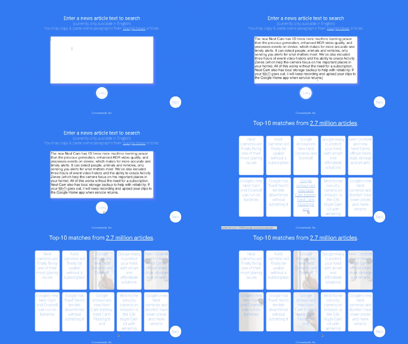
Vector Search: the technology behind Google Search, YouTube, Play, and more
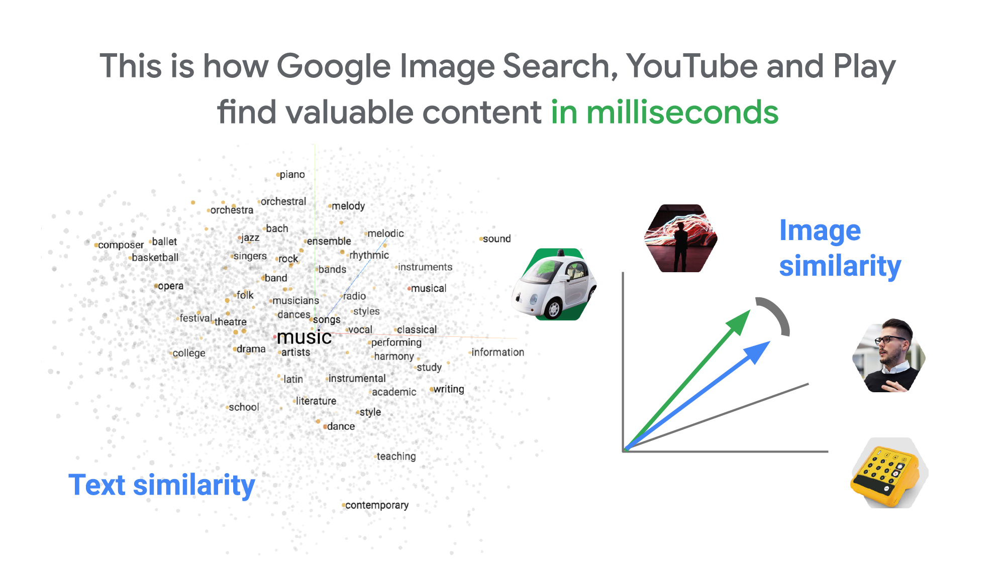
How can it find matches that fast? The trick is that the MatchIt Fast demo uses the vector similarity search (or nearest neighbor search or simply vector search) capabilities of the Vertex AI Matching Engine, which shares the same backend as Google Image Search, YouTube, Google Play, and more, for billions of recommendations and information retrievals for Google users worldwide. The technology is one of the most important components of Google’s core services, and not just for Google: it is becoming a vital component of many popular web services that rely on content search and information retrieval accelerated by the power of deep neural networks.
So what’s the difference between traditional keyword-based search and vector similarity search? For many years, relational databases and full-text search engines have been the foundation of information retrieval in modern IT systems. For example, you would add tags or category keywords such as “movie”, “music”, or “actor” to each piece of content (image or text) or each entity (a product, user, IoT device, or anything really). You’d then add those records to a database, so you could perform searches with those tags or keywords.
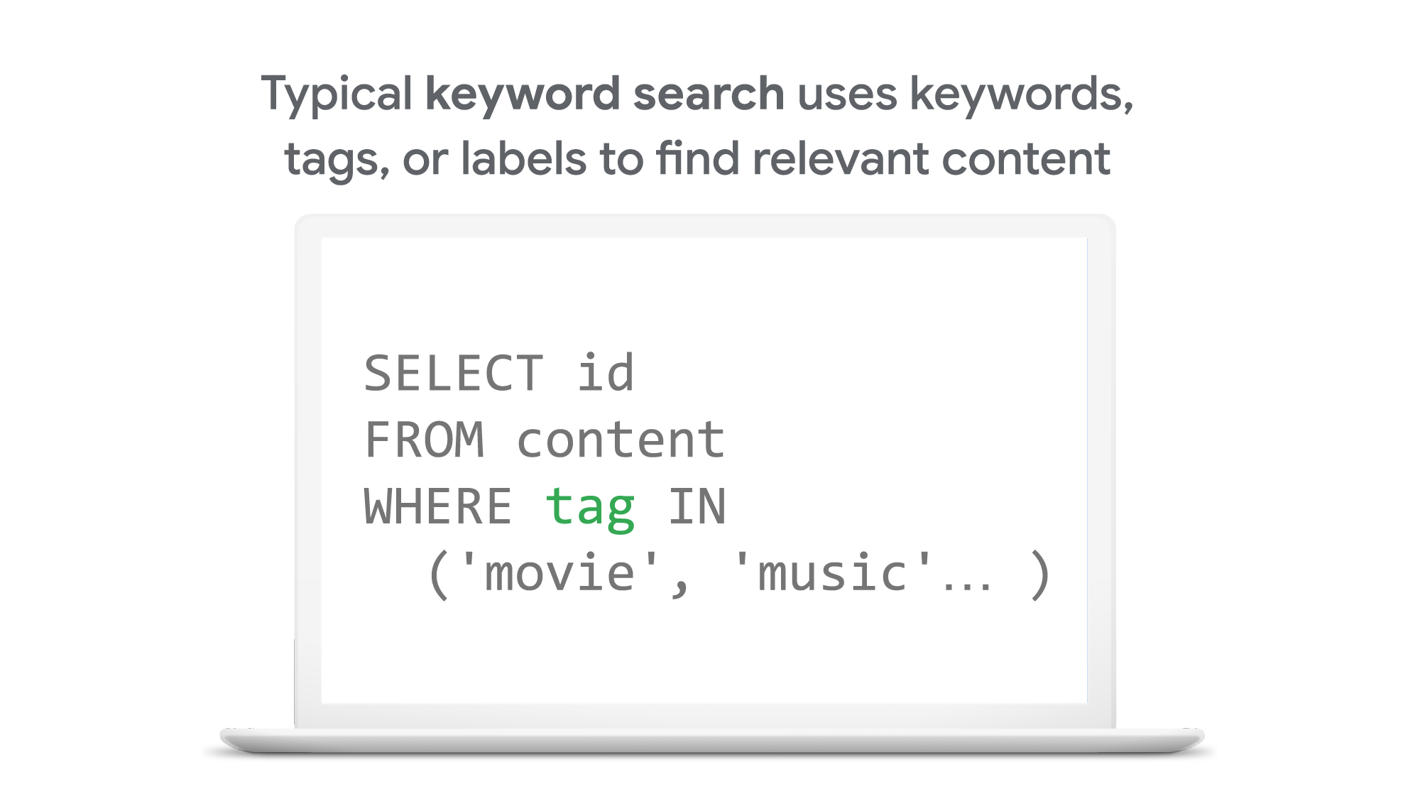
In contrast, vector search uses vectors (where each vector is a list of numbers) for representing and searching content. The combination of the numbers defines similarity to specific topics. For example, if an image (or any content) includes 10% of “movie”, 2% of “music”, and 30% of “actor”-related content, then you could define a vector [0.1, 0.02, 0.3] to represent it. (Note: this is an overly simplified explanation of the concept; the actual vectors have much more complex vector spaces). You can find similar content by comparing the distances and similarities between vectors. This is how Google services find valuable content for a wide variety of users worldwide in milliseconds.
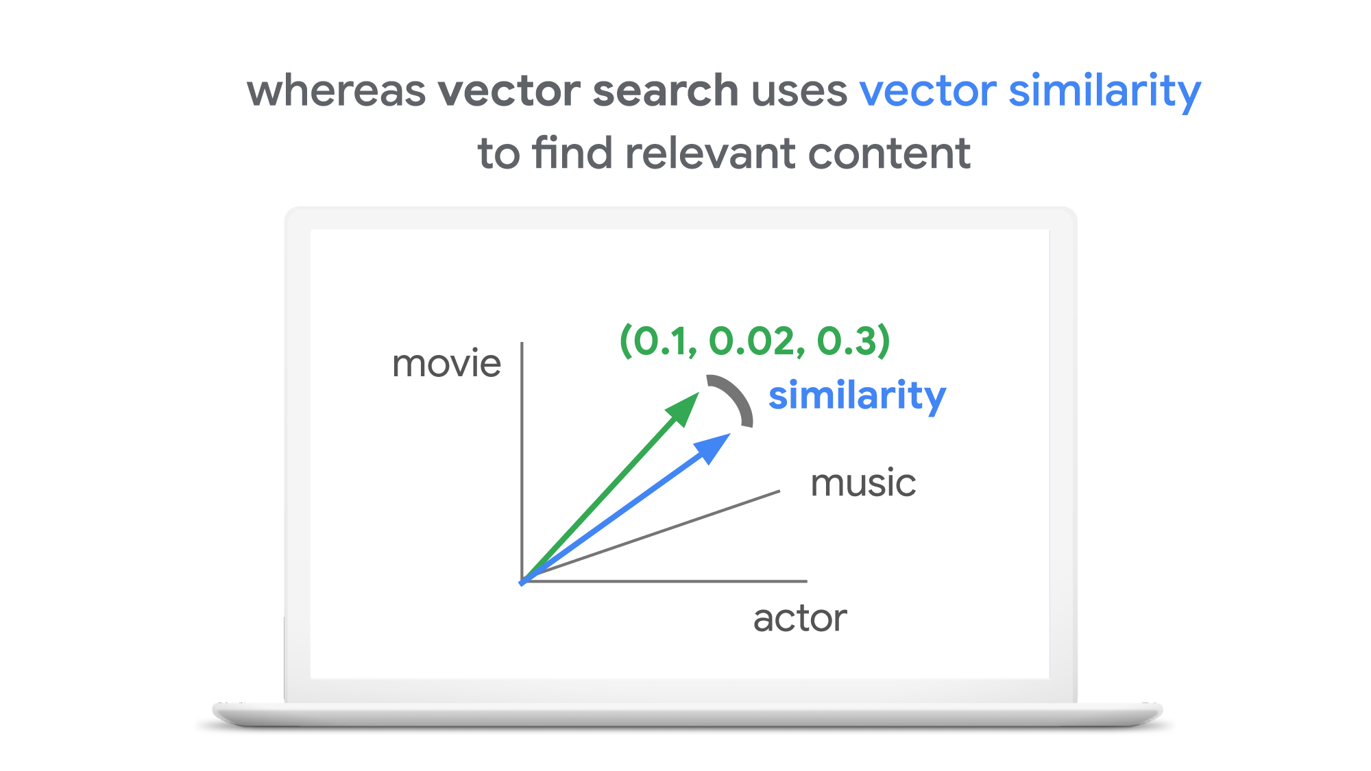
With keyword search, you can only specify a binary choice as an attribute of each piece of content; it’s either about a movie or not, either music or not, and so on. Also, you cannot express the actual “meaning” of the content to search. If you specify a keyword “films”, for example, you would not see any content related to “movies” unless there was a synonyms dictionary that explicitly linked these two terms in the database or search engine.
Vector search provides a much more refined way to find content, with subtle nuances and meanings. Vectors can represent a subset of content that contains “much about actors, some about movies, and a little about music”. Vectors can represent the meaning of content where “films”, “movies”, and “cinema” are all collected together. Also, vectors have the flexibility to represent categories previously unknown to or undefined by service providers. For example, emerging categories of content primarily attractive to kids, such as ASMR or slime, are really hard for adults or marketing professionals to predict beforehand, and going back through vast databases to manually update content with these new labels would be all but impossible to do quickly. But vectors can capture and represent never-before-seen categories instantly.
Vector search changes business
Vector search is not only applicable to image and text content. It can also be used for information retrieval for anything you have in your business when you can define a vector to represent each thing. Here are a few examples:
- Finding similar users: If you define a vector to represent each user in your business by combining the user’s activities, past purchase history, and other user attributes, then you can find all users similar to a specified user. You can then see, for example, users who are purchasing similar products, users that are likely bots, or users who are potential premium customers and who should be targeted with digital marketing.
- Finding similar products or items: With a vector generated from product features such as description, price, sales location, and so on, you can find similar products to answer any number of questions; for example, “What other products do we have that are similar to this one and may work for the same use case?” or “What products sold in the last 24 hours in this area?” (based on time and proximity)
- Finding defective IoT devices: With a vector that captures the features of defective devices from their signals, vector search enables you to instantly find potentially defective devices for proactive maintenance.
- Finding ads: Well-defined vectors let you find the most relevant or appropriate ads for viewers in milliseconds at high throughput.
- Finding security threats: You can identify security threats by vectorizing the signatures of computer virus binaries or malicious attack behaviors against web services or network equipment.
- …and many more: Thousands of different applications of vector search in all industries will likely emerge in the next few years, making the technology as important as relational databases.
OK, vector search sounds cool. But what are the major challenges to applying the technology to real business use cases? Actually there are two:
- Creating vectors that are meaningful for business use cases
- Building a fast and scalable vector search service
Embeddings: meaningful vectors for business use cases
The first challenge is creating vectors for representing various entities that are meaningful and useful for business use cases. This is where deep learning technology can really shine. In the case of the MatchIt Fast demo, the application simply uses a pre-trained MobileNet v2 model for extracting vectors from images, and the Universal Sentence Encoder (USE) for text. By applying such models to raw data, you can extract “embeddings” – vectors that map each row of data in a space of their “meanings”. MobileNet puts images that have similar patterns and textures closer to one another in the embedding space, and USE puts texts that have similar topics closer.
For example, a carefully designed and trained machine learning model could map movies into an embedding space like the following:
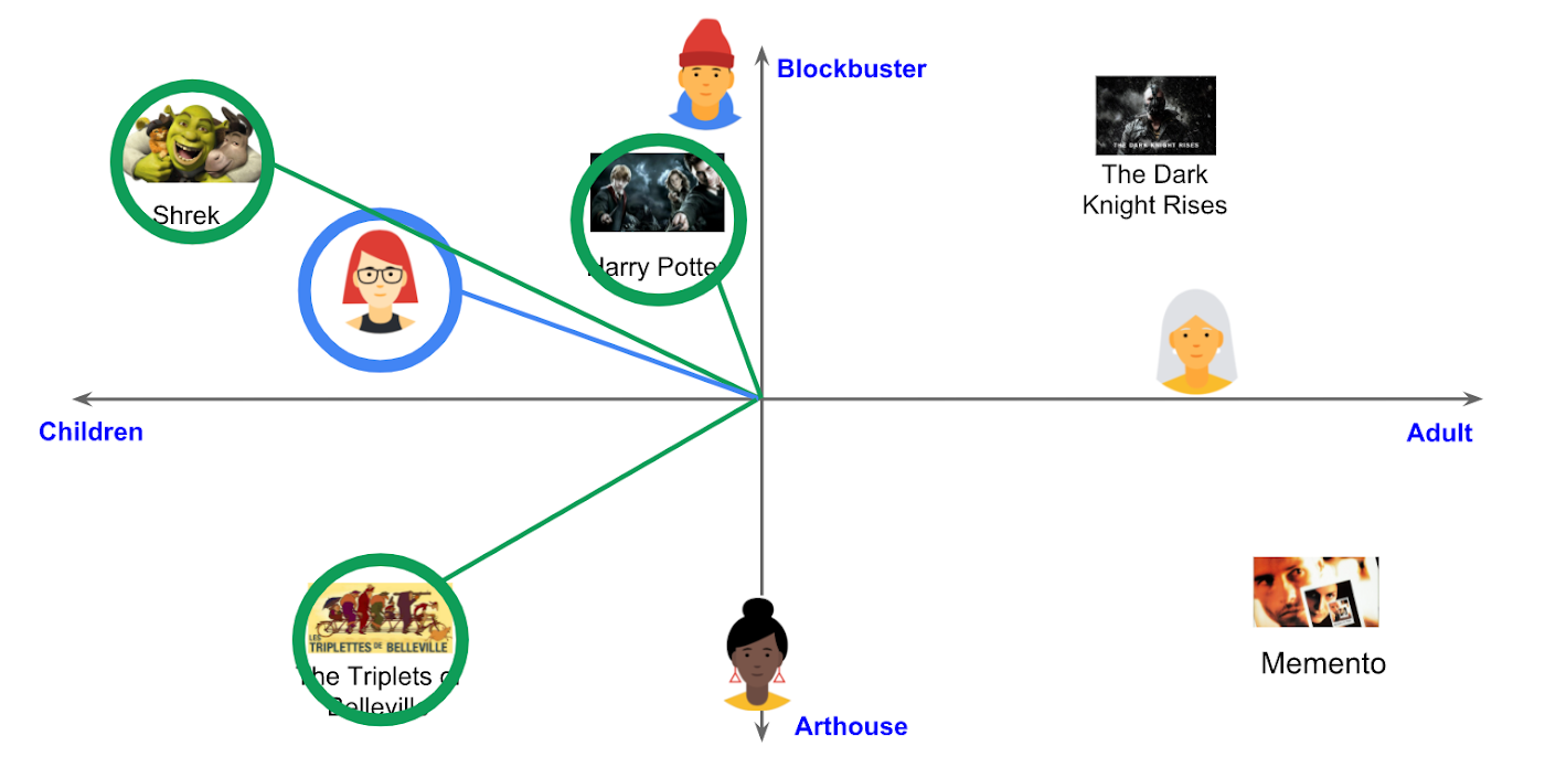
With the embedding space shown here, users could find recommended movies based on the two dimensions: is the movie for children or adults, and is it a blockbuster or arthouse movie? This is a very simple example, of course, but with an embedding space like this that fits your business requirements, you can deliver a better user experience on recommendation and information retrieval services with insights extracted from the model.
For more about creating embeddings, the Machine Learning Crash Course on Recommendation Systems is a great way to get started. We will also discuss how to extract better embeddings from business data later in this post.
Building a fast and scalable vector search service
Suppose that you have successfully extracted useful vectors (embeddings) from your business data. Now the only thing you have to do is search for similar vectors. That sounds simple, but in practice it is not. Let’s see how the vector search works when you implement it with BigQuery in a naive way:https://www.youtube.com/embed/wHNJspvxj2w?enablejsapi=1&
It takes about 20 seconds to find similar items (fish images in this case) from a pool of one million items. That level of performance is not so impressive, especially when compared to the MatchIt Fast demo. BigQuery is one of the fastest data warehouse services in the industry, so why does the vector search take so long?
This illustrates the second challenge: building a fast and scalable vector search engine isn’t an easy task. The most widely used metrics for calculating the similarity between vectors are L2 distance (Euclidean distance), cosine similarity, and inner product (dot product).
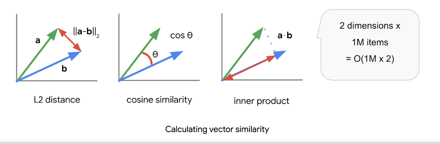
But all require calculations proportional to the number of vectors multiplied by the number of dimensions if you implement them in a naive way. For example, if you compare a vector with 1024 elements to 1M vectors, the number of calculations will be proportional to 1024 x 1M = 1.02B. This is the computation required to look through all the entities for a single search, and the reason why the BigQuery demo above takes so long.
Instead of comparing vectors one by one, you could use the approximate nearest neighbor (ANN) approach to improve search times. Many ANN algorithms use vector quantization (VQ), in which you split the vector space into multiple groups, define “codewords” to represent each group, and search only for those codewords. This VQ technique dramatically enhances query speeds and is the essential part of many ANN algorithms, just like indexing is the essential part of relational databases and full-text search engines.
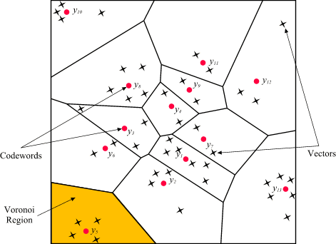
As you may be able to conclude from the diagram above, as the number of groups in the space increases the speed of the search decreases and the accuracy increases. Managing this trade-off — getting higher accuracy at shorter latency — has been a key challenge with ANN algorithms.
Last year, Google Research announced ScaNN, a new solution that provides state-of-the-art results for this challenge. With ScaNN, they introduced a new VQ algorithm called anisotropic vector quantization:
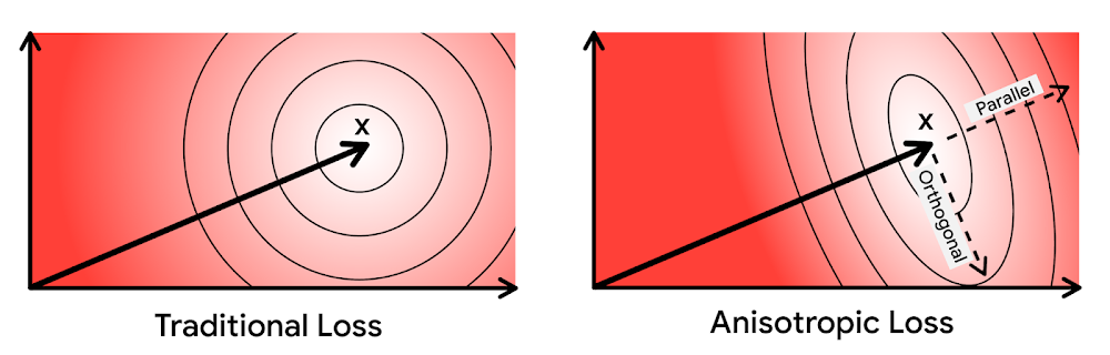
Anisotropic vector quantization uses a new loss function to train a model for VQ for an optimal grouping to capture farther data points (i.e. higher inner product) in a single group. With this idea, the new algorithm gives you higher accuracy at lower latency, as you can see in the benchmark result below (the violet line):
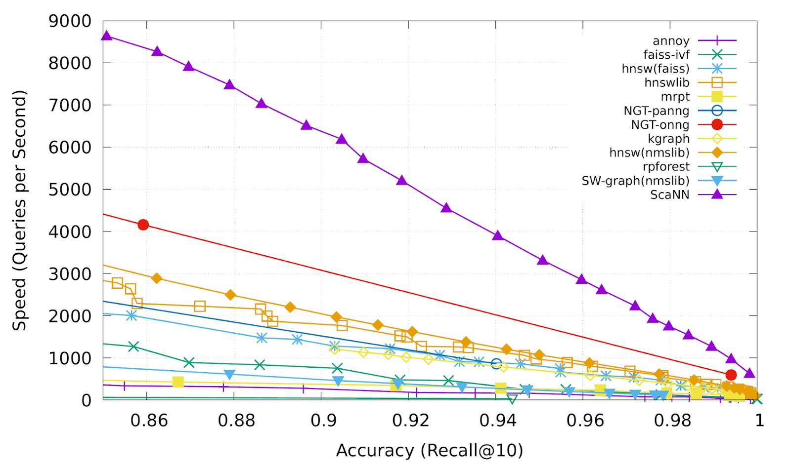
This is the magic ingredient in the user experience you feel when you are using Google Image Search, YouTube, Google Play, and many other services that rely on recommendations and search. In short, Google’s ANN technology enables users to find valuable information in milliseconds, in the vast sea of web content.
How to use Vertex AI Matching Engine
Now you can use the same search technology that powers Google services with your own business data. Vertex AI Matching Engine is the product that shares the same ScaNN based backend with Google services for fast and scalable vector search, and recently it became GA and ready for production use. In addition to ScaNN, Matching Engine gives you additional features as a commercial product, including:
- Scalability and availability: The open source version of ScaNN is a good choice for evaluation purposes, but as with most new and advanced technologies, you can expect challenges when putting it into production on your own. For example, how do you operate it on multiple nodes with high scalability, availability, and maintainability? Matching Engine uses Google’s production backend for ScaNN, which provides auto-scaling and auto-failover with a large worker pool. It is capable of handling tens of thousands of requests per second, and returns search results in less than 10 ms for the 90th percentile with a recall rate of 95 – 98%.
- Fully managed: You don’t have to worry about building and maintaining the search service. Just create or update an index with your vectors, and you will have a production-ready ANN service deployed. No need to think about rebuilding and optimizing indexes, or other maintenance tasks.
- Filtering: Matching Engine provides filtering functionality that enables you to filter search results based on tags you specify on each vector. For example, you can assign “country” and “stocked” tags to each fashion item vector, and specify filters like “(US OR Canada) AND stocked” or “not Japan AND stocked” on your searches.
Let’s see how to use Matching Engine with code examples from the MatchIt Fast demo.
Generating embeddings
Before starting the search, you need to generate embeddings for each item like this one:
{"Id":"b5c65fea9b0b8a57bfa574ea","Embedding": [0.16329009830951691,0.92436742782592773,0.00095699273515492678,0.011479727923870087,0.0089491046965122223,0.019959751516580582,0.031516745686531067,0.0066015380434691906,0.46404418349266052,...
This is an embedding with 1280 dimensions for a single image, generated with a MobileNet v2 model. The MatchIt Fast demo generates embeddings for two million images with the following code:
class Vectorizer:def __init__(self):self._model = tf.keras.Sequential([hub.KerasLayer("https://tfhub.dev/google/imagenet/mobilenet_v2_100_224/feature_vector/5", trainable=False)])self._model.build([None, 224, 224, 3]) # Batch input shape.def vectorize(self, jpeg_file):...snip...embedding = self._model.predict({"inputs": input_tensor})[0].tolist()return embedding
After you generate the embeddings, you store them in a Google Cloud Storage bucket.
Configuring an index
Then, define a JSON file for the index configuration:
{"contentsDeltaUri": "gs://match-it-fast-us-central1/wikimedia_images/index-1","config": {"dimensions": 1280,"approximateNeighborsCount": 150,"distanceMeasureType": "SQUARED_L2_DISTANCE","algorithm_config": {"treeAhConfig": {"leafNodeEmbeddingCount": 1000,"leafNodesToSearchPercent": 5}}}}
You can find a detailed description for each field in the documentation, but here are some important fields:
contentsDeltaUri: the place where you have stored the embeddingsdimensions: how many dimensions in the embeddingsapproximateNeighborsCount: the default number of neighbors to find via approximate searchdistanceMeasureType: how the similarity between embeddings should be measured, either L1, L2, cosine or dot product (this page explains which one to choose for different embeddings)
To create an index on the Matching Engine, run the following gcloud command where the metadata-file option takes the JSON file name defined above.
gcloud --project=gn-match-it-fast beta ai indexes create \--display-name=wikimedia-images \--description="Wikimedia Image Demo" \--metadata-file=metadata/wikimedia_images_index_metadata.json \--region=us-central1
Run the search
Now the Matching Engine is ready to run. The demo processes each search request in the following order:
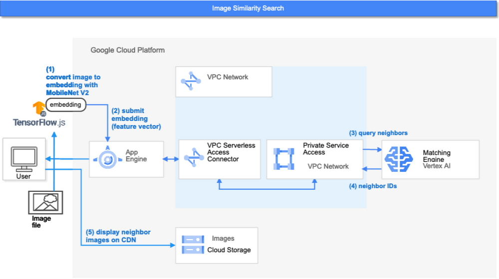
- First, the web UI takes an image (the one chosen or uploaded by the user) and encodes it into an embedding using the TensorFlow.js MobileNet v2 model running inside the browser. Note: this “client-side encoding” is an interesting option for reducing network traffic when you can run the encoding at the client. In many other cases, you would encode contents to embeddings with a server-side prediction service such as Vertex AI Prediction, or just retrieve pre-generated embeddings from a repository like Vertex AI Feature Store.
- The App Engine frontend receives the embedding and submits a query to the Matching Engine. Note that you can also use any other compute services in Google Cloud for submitting queries to Matching Engine, such as Cloud Run, Compute Engine, or Kubernetes Engine, or whatever is most suitable for your applications.
- Matching Engine executes its search. The connection between App Engine and Matching Engine is provided via a VPC private network for optimal latency.
- Matching Engine returns the IDs of similar vectors in its index.
Step 3 is implemented with the following code:
class MatchingQueryClient:...snip...def query_embedding(self, embedding, num_neighbors=30):request = match_service_pb2.MatchRequest()request.deployed_index_id = self._deployed_index_idfor v in embedding:request.float_val.append(v)request.num_neighbors = num_neighborsresponse = self._stub.Match(request)return response
The request to the Matching Engine is sent via gRPC as you can see in the code above. After it gets the request object, it specifies the index id, appends elements of the embedding, specifies the number of neighbors (similar embeddings) to retrieve, and calls the Match function to send the request. The response is received within milliseconds.
Next steps: Making changes for various use cases and better search quality
As we noted earlier, the major challenges in applying vector search on production use cases are:
- Creating vectors that are meaningful for business use cases
- Building a fast and scalable vector search service
From the example above, you can see that Vertex AI Matching Engine solves the second challenge. What about the first one? Matching Engine is a vector search service; it doesn’t include the creating vectors part.
The MatchIt Fast demo uses a simple way of extracting embeddings from images and contents; specifically it uses an existing pre-trained model (either MobileNet v2 or Universal Sentence Encoder). While those are easy to get started with, you may want to explore other options to generate embeddings for other use cases and better search quality, based on your business and user experience requirements.
For example, how do you generate embeddings for product recommendations? The Recommendation Systems section of the Machine Learning Crash Course is a great resource for learning how to use collaborative filtering and DNN models (the two-tower model) to generate embeddings for recommendation. Also, TensorFlow Recommenders provides useful guides and tutorials for the topic, especially on the two-tower model and advanced topics. For integration with Matching Engine, you may also want to check out the Train embeddings by using the two-tower built-in algorithm page.
Another interesting solution is the Swivel model. Swivel is a method for generating item embeddings from an item co-occurrence matrix. For structured data, such as purchase orders, the co-occurrence matrix of items can be computed by counting the number of purchase orders that contain both product A and product B, for all products you want to generate embeddings for. To learn more, take a look at this tutorial on how to use the model with Matching Engine.
If you are looking for more ways to achieve better search quality, consider metric learning, which enables you to train a model for discrimination between entities in the embedding space, not only classification:
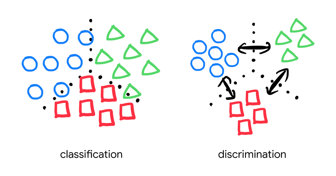
Popular pre-trained models such as the MobileNet v2 can classify each object in an image, but they are not explicitly trained to discriminate the objects from each other with a defined distance metric. With metric learning, you can expect better search quality by designing the embedding space optimized for various business use cases. TensorFlow Similarity could be an option for integrating metric learning with Matching Engine.
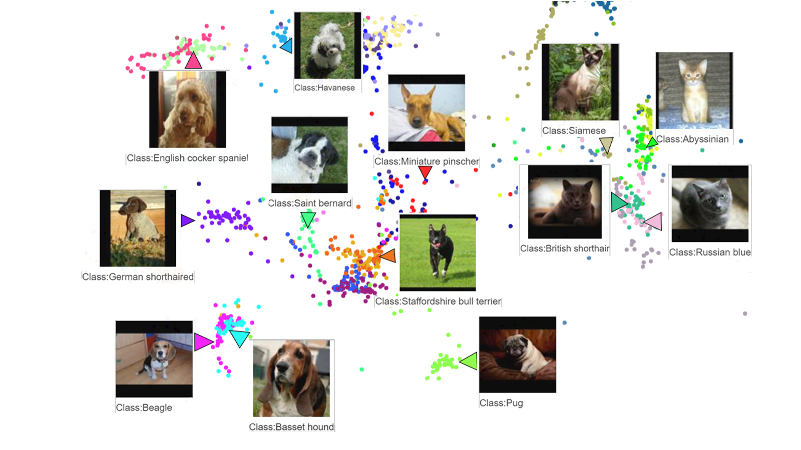
Interested? Today, we’re just beginning the migration from traditional search technology to new vector search. Over the next 5 to 10 years, many more best practices and tools will be developed in the industry and community. These tools and best practices will help answer many questions, like… How do you design your own embedding space for a specific business use case? How do you measure search quality? How do you debug and troubleshoot the vector search? How do you build a hybrid setup with existing search engines for meeting sophisticated requirements? There are many new challenges and opportunities ahead for introducing the technology to production. Now’s the time to get started delivering better user experiences and seizing new business opportunities with Matching Engine powered by vector search.
Acknowledgements
We would like to thank Anand Iyer, Phillip Sun, and Jeremy Wortz for their invaluable feedback to this post.
BigQuery Helps Insurance Firms Leverage Previous Storm Data for Better Pricing Insights

8554
Of your peers have already read this article.
2:00 Minutes
The most insightful time you'll spend today!
It may be surprising to know that U.S. natural catastrophe economic losses totaled $119 billion in 2020, and 75% (or $89.4B) of those economic losses were caused by severe storms and cyclones. In the insurance industry, data is everything. Insurers use data to influence underwriting, rating, pricing, forms, marketing, and even claims handling. When fueled by good data, risk assessments become more accurate and produce better business results. To make this possible, the industry is increasingly turning to predictive analytics, which uses data, statistical algorithms, and machine learning (ML) techniques to predict future outcomes based on historical data. Insurance firms also integrate external data sources with their own existing data to generate more insight into claimants and damages. Google Cloud Public Datasets offers more than 100 high-demand public datasets through BigQuery that helps insurers in these sorts of data “mashups.”
One particular dataset that insurers find very useful is Severe Storm Event Details from the U.S. National Oceanic and Atmospheric Administration (NOAA). As part of the Google Cloud Public Datasets program and NOAA’s Public Data Program, this severe storm data contains various types of storm reports by state, county, and event type—from 1950 to the present—with regular updates. Similar NOAA datasets within the Google Cloud Public Datasets program include the Significant Earthquake Database, Global Hurricane Tracks, and the Global Historical Tsunami Database.
In this post, we’ll explore how to apply storm event data for insurance pricing purposes using a few common data science tools—Python Notebook and BigQuery—to drive better insights for insurers.
Predicting outcomes with severe storm datasets
For property insurers, common determinants of insurance pricing include home condition, assessor and neighborhood data, and cost-to-replace. But macro forces such as natural disasters—like regional hurricanes, flash floods, and thunderstorms—can also significantly contribute to the risk profile of the insured. Insurance companies can leverage severe weather data for dynamic pricing of premiums by analyzing the severity of those events in terms of past damage done to property and crops, for example.
It’s important to set the premium correctly, however, considering the risks involved. Insurance companies now run sophisticated statistical models, taking into account various factors—many of which can change over time. After all, without accurate data, poor predictions can lead to business losses, particularly at scale.
The Severe Storm Event Details database includes information about a storm event’s location, azimuth (an angle measurement used in celestial coordination), distance, impact, and severity, including the cost of damages to property and crops. It documents:
- The occurrence of storms and other significant weather events of sufficient intensity to cause loss of life, injuries, significant property damage, and/or disruption to commerce.
- Rare, unusual weather events that generate media attention, such as snow flurries in South Florida or the San Diego coastal area.
- Other significant weather events, such as record maximum or minimum temperatures or precipitation that occur in connection with another event.
Data about a specific event is added to the dataset within 120 days to allow time for damage assessments and other analysis.
Driving business insights with BigQuery and notebooks
Google Cloud’s BigQuery provides easy access to this data in multiple ways. For example, you can query directly within BigQuery and perform analysis using SQL.
Another popular option in the data science and analyst community is to access BigQuery from within the Notebook environment to intersperse Python code and SQL text, and then perform ad hoc experimentation. This uses the powerful BigQuery compute to query and process huge amounts of data without having to perform the complex transformations within the memory in Pandas, for example.
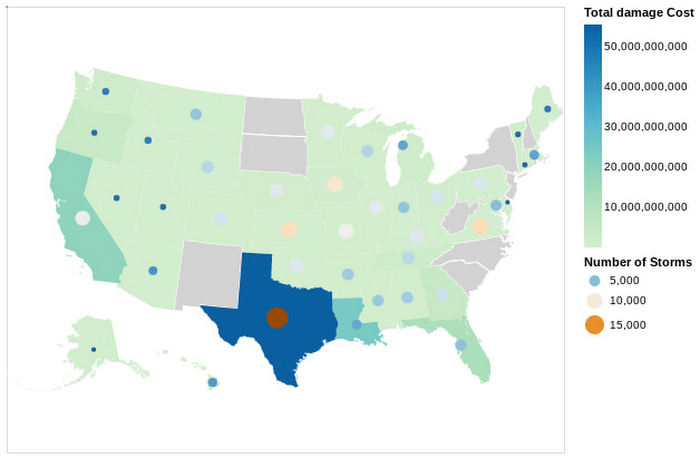
In this Python notebook, we have shown how the severe storm data can be used to generate risk profiles of various zip codes based on the severity of those events as measured by the damage incurred. The severe storm dataset is queried to retrieve a smaller dataset into the notebook, which is then explored and visualized using Python. Here’s a look at the risk profiles of the zip codes:
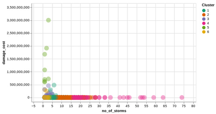
Another Google Cloud resource for insurers is BigQuery ML, which allows them to create and execute machine learning models on their data using standard SQL queries. In this notebook, with a K-Means Clustering algorithm, we have used BigQuery ML to generate different clusters of zip codes in the top five states impacted by severe storms. These clusters show different levels of impact by the storms, indicating different risk groups.
The example notebook is a reference guide to enable analysts to easily incorporate and leverage public datasets to augment their analysis and streamline the journey to business insights. Instead of having to figure out how to access and use this data yourself, the public datasets, coupled with BigQuery and other solutions, provide a well-lit path to insights, leaving you more time to focus on your own business solutions.
Making an impact with big data
Google Cloud’s Public Datasets is just one resource within the broader Google Cloud ecosystem that provides data science teams within the financial services with flexible tools to gather deeper insights for growth. The severe storm dataset is a part of our environmental, social, and governance (ESG) efforts to organize information about our planet and make it actionable through technology, helping people make a positive impact together.
To learn more about this public dataset collaboration between Google Cloud and NOAA, attend the Dynamic Pricing in Insurance: Leveraging Datasets To Predict Risk and Price session at the Google Cloud Financial Services Summit on May 27. You can also check out our recent blog and explore more about BigQuery and BigQuery ML.
New Capabilities in BigQuery to Ease Anomalies Detection in the Absence of Labeled Data

6323
Of your peers have already read this article.
4:00 Minutes
The most insightful time you'll spend today!
When it comes to anomaly detection, one of the key challenges that many organizations face is that it can be difficult to know how to define what an anomaly is. How do you define and anticipate unusual network intrusions, manufacturing defects, or insurance fraud? If you have labeled data with known anomalies, then you can choose from a variety of supervised machine learning model types that are already supported in BigQuery ML. But what can you do if you don’t know what kind of anomaly to expect, and you don’t have labeled data? Unlike typical predictive techniques that leverage supervised learning, organizations may need to be able to detect anomalies in the absence of labeled data.
Today we are announcing the public preview of new anomaly detection capabilities in BigQuery ML that leverage unsupervised machine learning to help you detect anomalies without needing labeled data. Depending on whether or not the training data is time series, users can now detect anomalies in training data or on new input data using a new ML.DETECT_ANOMALIES function (documentation), with the following models:
- Autoencoder model, now in Public Preview (documentation)
- K-means model, already GA (documentation)
- ARIMA_PLUS time series model, already GA (documentation)
How does anomaly detection with ML.DETECT_ANOMALIES work?
To detect anomalies in non-time-series data, you can use:
- K-means clustering models: When you use
ML.DETECT_ANOMALIESwith a k-means model, anomalies are identified based on the value of each input data point’s normalized distance to its nearest cluster. If that distance exceeds a threshold determined by the contamination value provided by the user, the data point is identified as an anomaly. - Autoencoder models: When you use
ML.DETECT_ANOMALIESwith an autoencoder model, anomalies are identified based on the reconstruction error for each data point. If the error exceeds a threshold determined by the contamination value, it is identified as an anomaly.
To detect anomalies in time-series data, you can use:
- ARIMA_PLUS time series models: When you use
ML.DETECT_ANOMALIESwith an ARIMA_PLUS model, anomalies are identified based on the confidence interval for that timestamp. If the probability that the data point at that timestamp occurs outside of the prediction interval exceeds a probability threshold provided by the user, the datapoint is identified as an anomaly.
Below we show code examples of anomaly detection in BigQuery ML for each of the above scenarios.
Anomaly detection with a k-means clustering model
You can now detect anomalies using k-means clustering models, by running ML.DETECT_ANOMALIES to detect anomalies in the training data or in new input data. Begin by creating a k-means clustering model:
Language: SQL
CREATE MODEL `mydataset.my_kmeans_model`OPTIONS(MODEL_TYPE = 'kmeans',NUM_CLUSTERS = 8,KMEANS_INIT_METHOD = 'kmeans++') ASSELECT* EXCEPT(Time, Class)FROM`bigquery-public-data.ml_datasets.ulb_fraud_detection`;
With the k-means clustering model trained, you can now run ML.DETECT_ANOMALIES to detect anomalies in the training data or in new input data.
To detect anomalies in the training data, use ML.DETECT_ANOMALIES with the same data used during training:
Language: SQL
SELECT*FROMML.DETECT_ANOMALIES(MODEL `mydataset.my_kmeans_model`,STRUCT(0.02 AS contamination),TABLE `bigquery-public-data.ml_datasets.ulb_fraud_detection`);
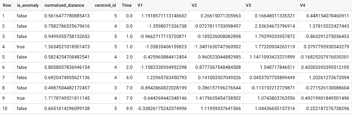
To detect anomalies in new data, use ML.DETECT_ANOMALIES and provide new data as input:
Language: SQL
SELECT*FROMML.DETECT_ANOMALIES(MODEL `mydataset.my_kmeans_model`,STRUCT(0.02 AS contamination),(SELECT * FROM `mydataset.newdata`));

How does anomaly detection work for k-means clustering models?
Anomalies are identified based on the value of each input data point’s normalized distance to its nearest cluster, which, if exceeds a threshold determined by the contamination value, is identified as an anomaly. How does this work exactly? With a k-means model and data as inputs, ML.DETECT_ANOMALIES first computes the absolute distance for each input data point to all cluster centroids in the model, then normalizes each distance by the respective cluster radius (which is defined as the standard deviation of the absolute distances of all points in this cluster to the centroid). For each data point, ML.DETECT_ANOMALIES returns the nearest centroid_id based on normalized_distance, as seen in the screenshot above. The contamination value, specified by the user, determines the threshold of whether a data point is considered an anomaly. For example, a contamination value of 0.1 means that the top 10% of descending normalized distance from the training data will be used as the cut-off threshold. If the normalized distance for a datapoint exceeds the threshold, then it is identified as an anomaly. Setting an appropriate contamination will be highly dependent on the requirements of the user or business.
For more information on anomaly detection with k-means clustering, please see the documentation here.
Anomaly detection with an autoencoder model
You can now detect anomalies using autoencoder models, by running ML.DETECT_ANOMALIES to detect anomalies in the training data or in new input data.
Begin by creating an autoencoder model:
Language: SQL
CREATE MODEL `mydataset.my_autoencoder_model`OPTIONS(model_type='autoencoder',activation_fn='relu',batch_size=8,dropout=0.2,hidden_units=[32, 16, 4, 16, 32],learn_rate=0.001,l1_reg_activation=0.0001,max_iterations=10,optimizer='adam') ASSELECT* EXCEPT(Time, Class)FROM`bigquery-public-data.ml_datasets.ulb_fraud_detection`;
To detect anomalies in the training data, use ML.DETECT_ANOMALIES with the same data used during training:
Language: SQL
SELECT*FROMML.DETECT_ANOMALIES(MODEL `mydataset.my_autoencoder_model`,STRUCT(0.02 AS contamination),TABLE `bigquery-public-data.ml_datasets.ulb_fraud_detection`);
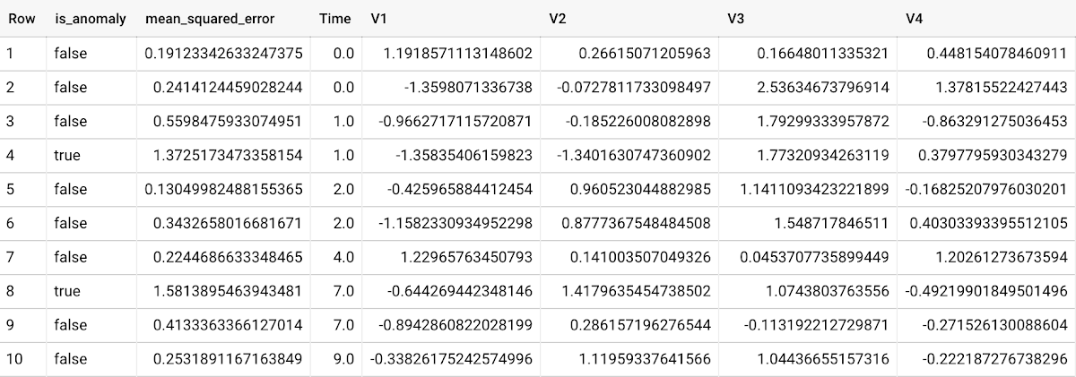
To detect anomalies in new data, use ML.DETECT_ANOMALIES and provide new data as input:
Language: SQL
SELECT*FROMML.DETECT_ANOMALIES(MODEL `mydataset.my_autoencoder_model`,STRUCT(0.02 AS contamination),(SELECT * FROM `mydataset.newdata`));

How does anomaly detection work for autoencoder models?
Anomalies are identified based on the value of each input data point’s reconstructed error, which, if exceeds a threshold determined by the contamination value, is identified as an anomaly. How does this work exactly? With an autoencoder model and data as inputs, ML.DETECT_ANOMALIES first computes the mean_squared_error for each data point between its original values and its reconstructed values. The contamination value, specified by the user, determines the threshold of whether a data point is considered an anomaly. For example, a contamination value of 0.1 means that the top 10% of descending error from the training data will be used as the cut-off threshold. Setting an appropriate contamination will be highly dependent on the requirements of the user or business.
For more information on anomaly detection with autoencoder models, please see the documentation here.
Anomaly detection with an ARIMA_PLUS time-series model
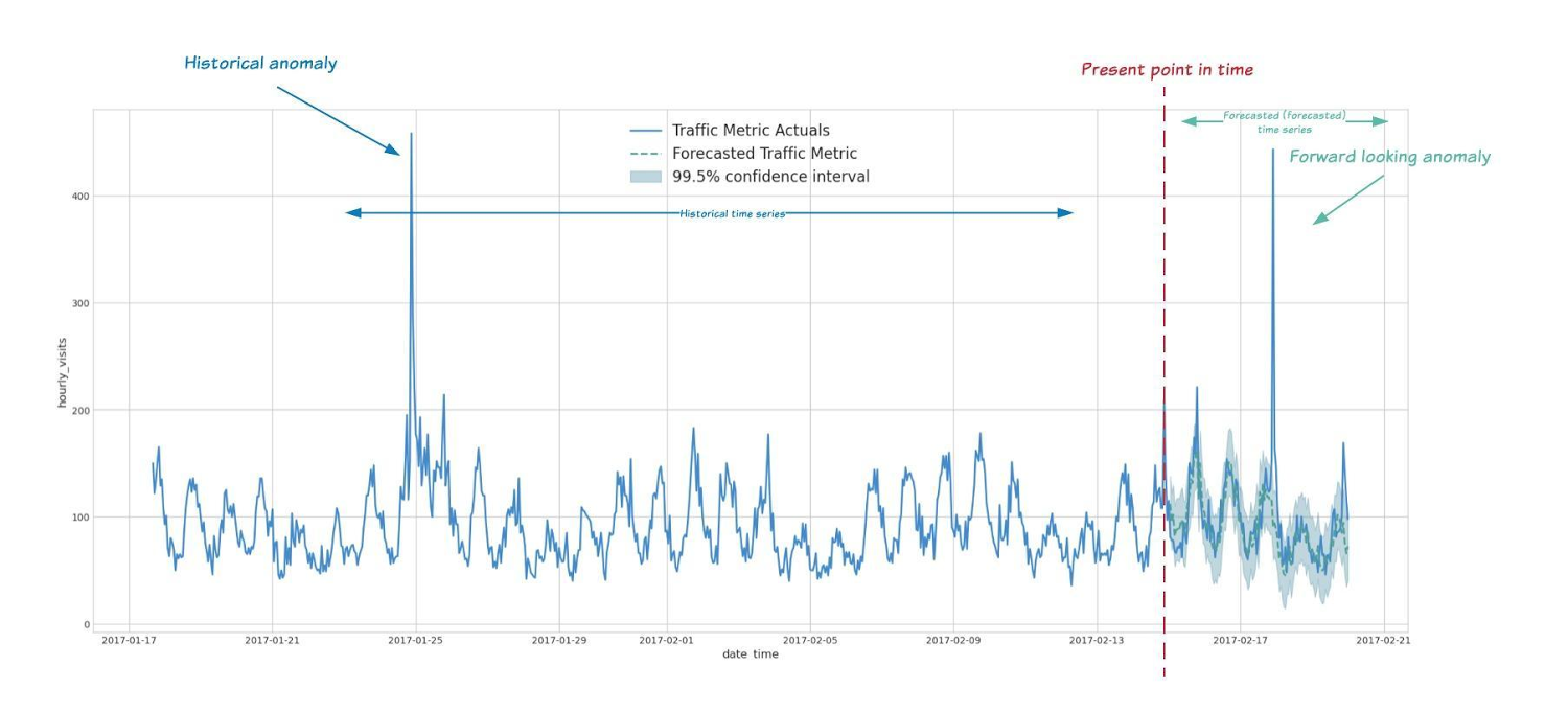
With ML.DETECT_ANOMALIES, you can now detect anomalies using ARIMA_PLUS time series models in the (historical) training data or in new input data. Here are some examples of when might you want to detect anomalies with time-series data:
Detecting anomalies in historical data:
- Cleaning up data for forecasting and modeling purposes, e.g. preprocessing historical time series before using them to train an ML model.
- When you have a large number of retail demand time series (thousands of products across hundreds of stores or zip codes), you may want to quickly identify which stores and product categories had anomalous sales patterns, and then perform a deeper analysis of why that was the case.
Forward looking anomaly detection:
- Detecting consumer behavior and pricing anomalies as early as possible: e.g. if traffic to a specific product page suddenly and unexpectedly spikes, it might be because of an error in the pricing process that leads to an unusually low price.
- When you have a large number of retail demand time series (thousands of products across hundreds of stores or zip codes), you would like to identify which stores and product categories had anomalous sales patterns based on your forecasts, so you can quickly respond to any unexpected spikes or dips.
How do you detect anomalies using ARIMA_PLUS? Begin by creating an ARIMA_PLUS time series model:
Language: SQL
CREATE OR REPLACE MODEL mydataset.my_arima_plus_modelOPTIONS(MODEL_TYPE='ARIMA_PLUS',TIME_SERIES_TIMESTAMP_COL='date',TIME_SERIES_DATA_COL='total_amount_sold',TIME_SERIES_ID_COL='item_name',HOLIDAY_REGION='US') ASSELECTdate,item_description AS item_name,SUM(bottles_sold) AS total_amount_soldFROM`bigquery-public-data.iowa_liquor_sales.sales`GROUP BYdate,item_nameHAVINGdate BETWEEN DATE('2016-01-04') AND DATE('2017-06-01')AND item_name IN ("Black Velvet", "Captain Morgan Spiced Rum","Hawkeye Vodka", "Five O'Clock Vodka", "Fireball Cinnamon Whiskey");
To detect anomalies in the training data, use ML.DETECT_ANOMALIES with the model obtained above:
Language: SQL
SELECT*FROMML.DETECT_ANOMALIES(MODEL `mydataset.my_arima_plus_model`,STRUCT(0.8 AS anomaly_prob_threshold));
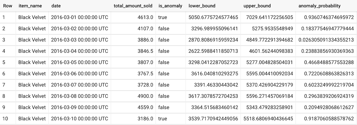
To detect anomalies in new data, use ML.DETECT_ANOMALIES and provide new data as input:
Language: SQL
WITHnew_data AS (SELECTdate,item_description AS item_name,SUM(bottles_sold) AS total_amount_soldFROM`bigquery-public-data.iowa_liquor_sales.sales`GROUP BYdate,item_nameHAVINGdate BETWEEN DATE('2017-06-02')AND DATE('2017-10-01')AND item_name IN ('Black Velvet','Captain Morgan Spiced Rum','Hawkeye Vodka',"Five O'Clock Vodka",'Fireball Cinnamon Whiskey') )SELECT*FROMML.DETECT_ANOMALIES(MODEL `mydataset.my_arima_plus_model`,STRUCT(0.8 AS anomaly_prob_threshold),(SELECT*FROMnew_data));
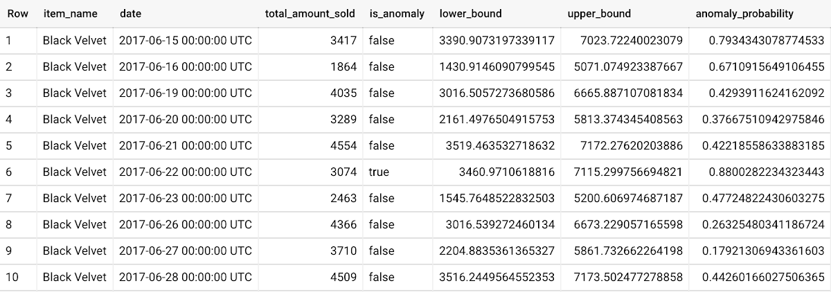
For more information on anomaly detection with ARIMA_PLUS time series models, please see the documentation here.
Thanks to the BigQuery ML team, especially Abhinav Khushraj, Abhishek Kashyap, Amir Hormati, Jerry Ye, Xi Cheng, Skander Hannachi, Steve Walker, and Stephanie Wang.
More Relevant Stories for Your Company

Quantum Metric Increases Business 10-fold
At Quantum Metric, we’re in the business of bringing our customers business insights that are based on customer experience data and analytics for mid-market and Fortune 500 companies. Our software, powered by big data, machine intelligence, and Google Cloud, helps our customers identify, quantify, prioritize and measure opportunities to improve

Google Cloud Celebrates Journey of 3 Inspiring Founders for the Asian Pacific American Heritage Month
May is Asian Pacific American Heritage Month —a time for us to come together to celebrate and remember the important people and history of Asian and Pacific Island heritage. This feature highlights three AAPI founders from the Google For Startups community. Read on to learn how these three founders built


Indian Retailer Figures Optimizes Hyperlocal Delivery to Increase Customer Experience
Anyone who follows the Indian e-commerce scene knows that one of the largest challenges these companies face is hyperlocal delivery. That was a problem facing Wellness Forever, a retail chain of pharmacies with 150-plus stores across India. “Exactly a year ago, we started our journey of hyperlocal deliveries. This optimization

The Right Datawarehouse Helps Fight Climate Change, While Improving Customer Experience
When you think about climate change, you might not consider a daily commute to work or a drive around town as big contributing factors. And yet, transport is the fastest growing source of CO2 emissions from fossil fuel, which in turn is the largest contributor to climate change. This is the key insight
