





Leverage the Power of Looker to Extract Data Value at Web Scale

4460
Of your peers have already read this article.
3:00 Minutes
The most insightful time you'll spend today!
Data science can be applied to business problems to improve practices and help to strengthen customer satisfaction. In this blog, we address how the addition of Looker extends the value of your Google Cloud investments to help you understand your customer journey, unlock value from first-party data, and optimize existing cloud infrastructure.
Data is a powerful tool
While everyone doesn’t need to understand the nuts and bolts of data technologies, most people do care about the value data can create for them — how it can help them do their jobs better. Within the data space, we are seeing a trend of ongoing failure to make data accessible to “humans” – the industry still hasn’t figured out how to put data into the hands of people when and where they need it, how they need it.
What if everyone in your organization could analyze data at scale, and make more-informed, fact-based decisions? Data and insights derived from data are valuable but only if your users see it. We think Looker helps solve that.
Solutions tell a larger story of how it all fits together
Across all verticals and industries, businesses benefit from knowing and understanding their customers better. Many business goals are to increase revenue by improving product recommendations and pricing optimization, improving the user experience through targeted marketing and personalization, and reducing churn while improving retention rates. To help reach these goals, key strategies should focus on understanding customer needs, their motivations, likes and dislikes, and using all available data – in other words, put yourself in the shoes of your customer.
Our goal with Looker solutions is to offer the right level of out-of-box support that allows customers to get to value quickly, while maintaining the necessary flexibility. We aim to offer a library of data-driven solutions that accelerate data projects. Many solutions include Looker Blocks (pre-built pieces of code that accelerate data exploration environments) and Actions (custom integrations) that get customers up and running quickly and lets you build business-friendly access points for Google Cloud functionality like BQML, App Engine and Cloud Functions.
Below, you’ll find a sampling of the newest Looker solutions.
Listening to customers by looking at the data
Looker’s solution for Contact Center AI (CCAI), helps businesses gain a deeper understanding and appreciation of their customers’ full journey by unlocking insights from all their company’s first-party data. Call centers can converse naturally with customers and deliver outstanding experiences by leveraging artificial intelligence. CCAI‘s newest product —CCAI Insights — reviews conversations support agents are having, finding and annotating the data with the important information, and identifying the calls that need review. We’ve partnered with the product teams at CCAI to build Looker’s Block for CCAI Insights, which sets you on the path to integrating the advanced insights into your first-party data in Looker, overlaying business data with the customer experience.

Businesses can better understand contact center experiences and take immediate action when necessary to make sure the most valuable customers receive the best service.
Realizing full business value of First-Party data
Looker for Google Marketing Platform (GMP) provides marketers the power to unlock the value of their company’s first-party data to more effectively target audiences. The Looker Blocks and Actions for GMP offer interactive data exploration, slices of data with built-in ML predictions and activation paths back to the GMP. This strategic solution continues to evolve with the Looker Action for Google Ads (Customer Match), the Looker Action for Google Analytics (Data Import) and the Looker Block for Google Analytics 4 (GA4).
- The Looker Action for Customer Match allows marketers to send segments and audiences based on first-party data directly into Google Ads. Reach users cross-device and across the web’s most powerful channels such as Display, Video, YouTube, and Gmail. The entire process is performed within a single screen in Looker, and is able to be completed in a few minutes by a non-technical user.
- The Looker Action for Data Import can be used to enhance user segmentation and remarketing audiences in Google Analytics by taking advantage of user information accessible in Looker, such as in CRM systems or transactional data warehouses.
- The Looker Block for Google Analytics 4 (GA4) expands the solution’s support with out-of-the-box dashboards and pre-baked BigQuery ML models for the newest version of Google Analytics.The Looker Block offers up reports with flexible configuration capabilities to unlock custom insights beyond the standard GA reporting. Customize audience segments, define custom goals to track and share these reports with teams who do not have access to the GA console.
From clinical notes to patient insights at scale
Taking a look at the Healthcare vertical, the Looker Healthcare NLP API Block serves as a critical bridge between existing care systems and applications hosted on Google Cloud providing a managed solution for storing and accessing healthcare data in Google Cloud. The Healthcare NLP API uses natural language models to extract healthcare information from medical text, rapidly unlocking insights from unstructured medical text and providing medical providers with simplified access to intelligent insights. Healthcare providers, payers, and pharma companies can quickly understand the context and relationships of medical concepts within the text, such as medications, procedures, conditions, clinical history, and begin to link this to other clinical data sources for downstream AI/ML.
Specifically, the natural language processing (NLP) Patient View (pictured below) allows you to review a single selected patient of interest, surfacing their clinical notes history over time. It informs clinical diagnosis with family history insights, which is not currently captured in claims, and captures additional procedure coding for revenue cycle purposes.

The dashboard below shows the NLP Term View which allows users to focus on chosen medical terms across the entire patient population in the dataset so they can start to view trends and patterns across groups of patients.

This data can be used to:
- Enhance patient matching for clinical trials
- Identify re-purposed medications
- Drive advancements for research in cancer and rare diseases
- Identify how social determinants of health impact access to care
Managing Costs Across Clouds
Effective cloud cost management is important for reasons beyond cost control — it provides you the ability to reduce waste and predictably forecast both costs and resource needs. Looker’s solution for Cloud Cost Management offers quick access to necessary reporting and clear insights into cloud expenditures and utilization.
This solution brings together billing data from different cloud providers in a phased approach: get up and running quickly with Blocks optimized for where the data is today (Google Cloud, AWS or Azure) as you work towards more sophisticated analysis for cross-platform planning and even cloud spend optimization with the mapping of tags, labels and cost centers across clouds.
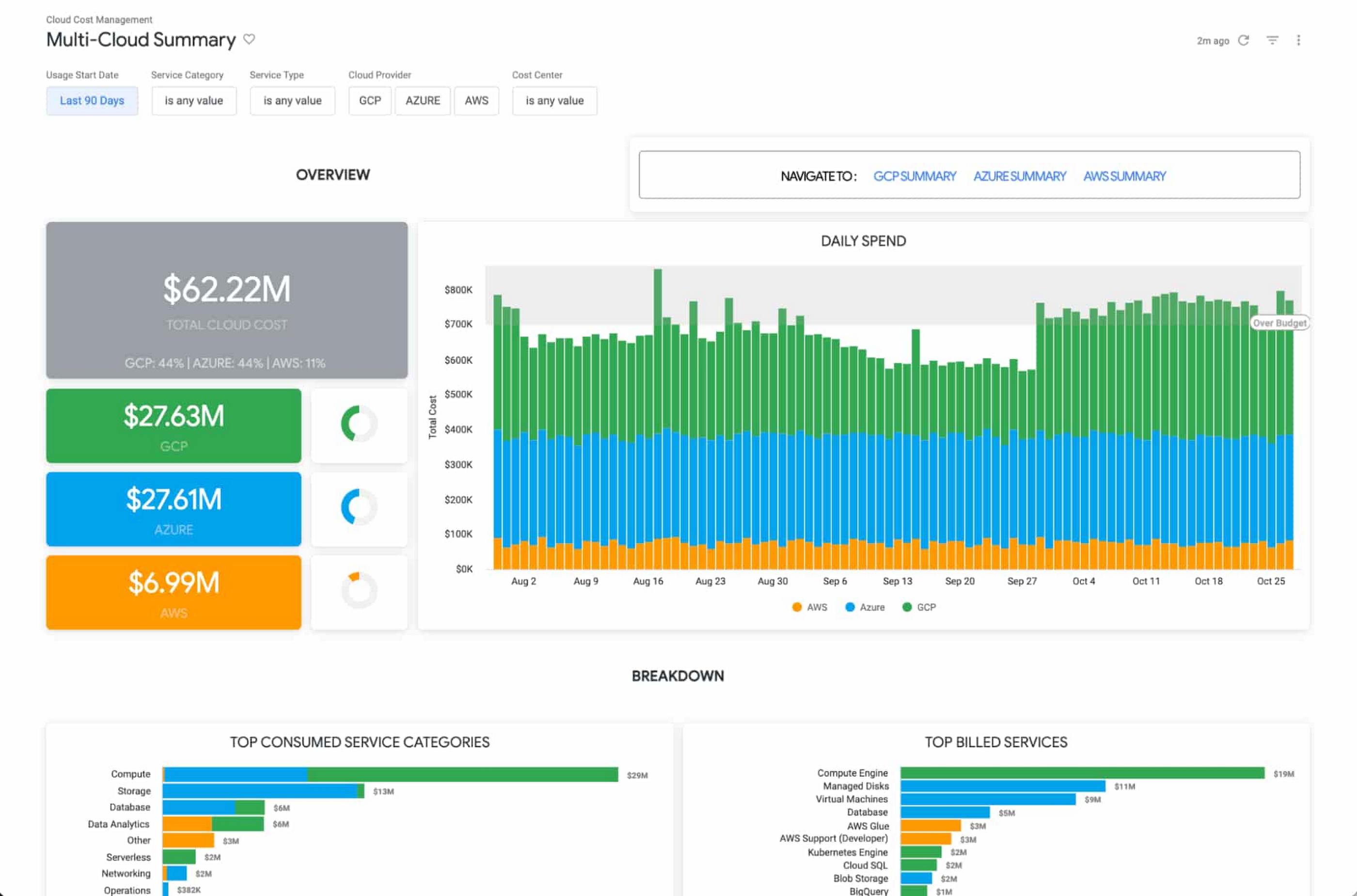
The Looker Cloud Cost Management solution provides operational teams struggling to monitor, understand, and manage the costs and needs associated with their cloud technology with a comprehensive view into what, where and why they are spending money.
Making better decisions with Looker-powered data
Leading companies are discovering ways to get value from all of that data beyond displaying it in a report or a dashboard. They want to enable everyone to make better decisions but that’s only going to happen if everyone can ask questions of the data, and get reliable, correct answers without using outdated or incomplete data and without waiting for it. People and systems need to have data available to them in the way that makes the most sense for them at that moment.
It’s clear that successful data-driven organizations will lead their respective segments not because they use data to create reports, but because they use it to power data experiences tailored to every part of the business, including employees, customers, operational workflows, products and services.
As people’s way of experiencing data has evolved, more than ever before, dashboards alone are not enough. You can use data as fuel for data-driven business workflows, and to power digital experiences that improve customer engagement, conversions, and advocacy.
From Nov. 9 – 11th, Looker is hosting its annual conference JOIN, where we’ll be showing new features, including how we help to:
- Build data experiences at the speed of business
- Accelerate the business value with packaged experiences
- Unleash more insights for more people in the right way – Deliver data experiences at scale
There is no cost to attend JOIN. Register here and learn how Looker helps organizations build and deliver custom data-driven experiences that goes beyond just reports and dashboards, scales and grows with your business, allows developers to build innovative data products faster, and ensures data reaches everyone.
Time-series Model on Google Cloud Allows Better Transparency on Fishing and Marine Activities

4407
Of your peers have already read this article.
3:30 Minutes
The most insightful time you'll spend today!
Who would have known that today technology would enable us with the ability to use machine learning to track vessel activity, and make pattern inferences to help address IUU (illegal, unreported, and unregulated) fishing activities. What’s even more noteworthy is that we now have the computing power to share this information publicly in order to enable fair and sustainable use of our ocean.
An amazing group of humans at the nonprofit Global Fishing Watch took on this massive big data challenge and succeeded. You can immediately access their dynamic map on their website globalfishingwatch.org/map that is bringing greater transparency to fishing activity and supporting the creation and management of marine protected areas throughout the world.
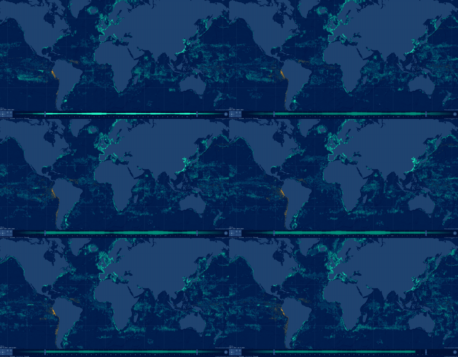
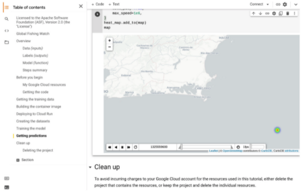
In our second episode of our People and Planet AI series we were inspired by their ML solution to this challenge, and we built a short video and sample with all the relevant code you need to get started with building a basic time-series classification model in Google Cloud, and visualize it in an interactive map.
Architecture
These are the components used to build a model for this sample:
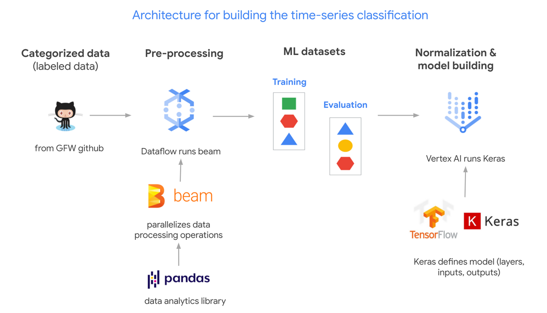
- Global Fishing Watch GitHub: where we got the data
- Apache Beam: (open source library) runs on Dataflow.
- Dataflow: (Google’s data processing service) creates 2 datasets; 1 for training a model and the other to evaluate its results.
- TensorflowKeras: (high level API library) used to define a machine learning model, which we then train in Vertex AI.
- Vertex AI: (a platform to build, deploy, and scale ML models) we train and output the model.
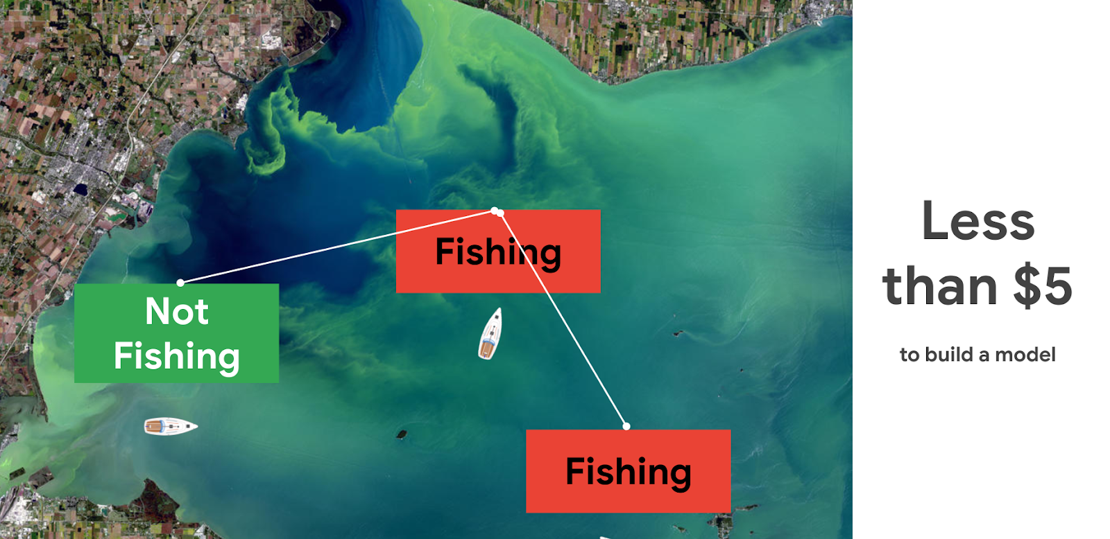
Pricing and steps
The total cost to run this solution was less than $5.
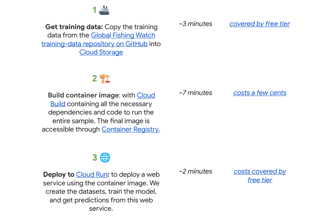
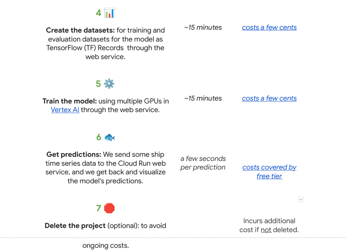
There are seven steps we went through with their approximate time and cost:
Why do we use a time series classification model?
Vessels in the ocean are constantly moving, which creates distinctive patterns from a satellite view.

We can train a model to recognize the shapes of a vessel’s trajectory. Large vessels are required to use the automatic identification system, or AIS. The GPS-like transponders regularly broadcast a vessel’s maritime mobile service identity, or MMSI, and other critical information to nearby ships, as well as to terrestrial and satellite receivers. While AIS is designed to prevent collisions and boost overall safety at sea, it has turned out to be an invaluable system for monitoring vessels and detecting suspicious fishing behavior globally.

One tricky part is that the MMSI data location signal (which includes a timestamp, latitude, longitude, distance from port, and more) is not emitted at regular intervals. AIS broadcast frequency changes with vessel speed (faster at higher speeds), and not all AIS messages that are broadcast are received – terrestrial receivers require line-of-sight, satellites must be overhead, and high vessel density can cause signal interference. For example, AIS messages might be received frequently as a vessel leaves the docks and operates near shore, then less frequently as they move further offshore until satellite reception improves. This is challenging for a machine learning model to interpret. There are too many gaps in the data, which makes it hard to predict.
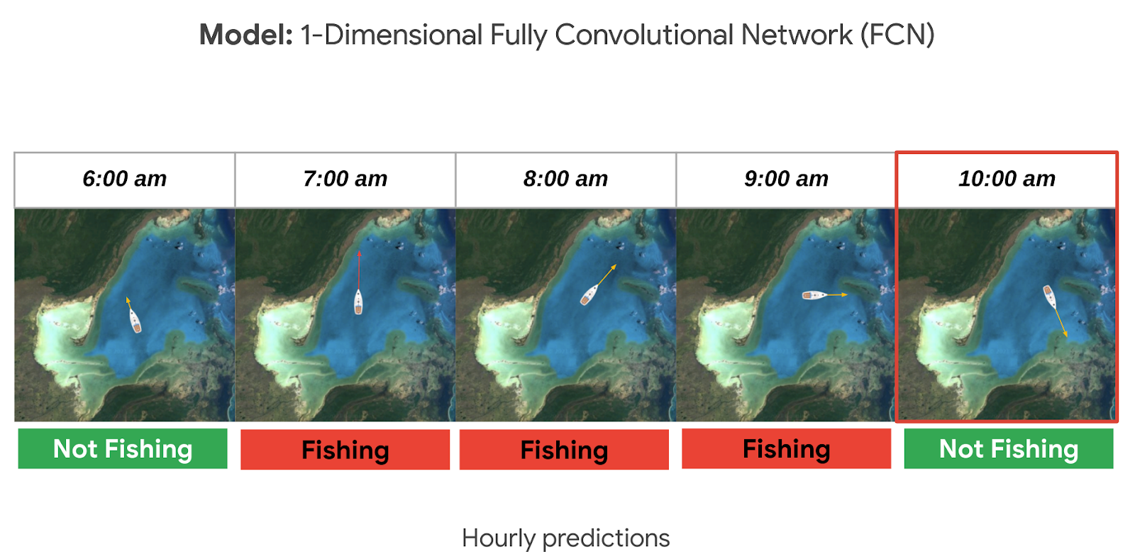
A way to solve this is to normalize the data and generate fixed-sized hourly windows. Then the model can predict if the vessel is fishing or not fishing for each hour.

It could be hard to know if a ship is fishing or not by just looking at its current position, speed, and direction. So we look at the data from the past as well, looking at the future could also be an option if we don’t need to do real time predictions. For this sample, it seemed reasonable to look 24 hours into the past to make a prediction. This means we need at least 25 hours of data to make a prediction for a single hour (24 hours in the past + 1 current hour). But we could predict longer time sequences as well. In general, to get hourly predictions, we need (n+24) hours of data.
Options to deploy and access the model
For this sample specifically we used Cloud Run to host the model as a web app so that other apps can call it to make predictions on an ongoing basis; this is our favorite in terms of pricing if you need to access your model from the internet over an extended period of time (charged per prediction request). You can also host it directly from Vertex AI where you trained and built the model, just note there is an hourly cost for using those VMs even if they are idle. If you do not need to access the model over the internet, you can make predictions locally or download the model onto a microcontroller if you have an IoT sensor strategy.

Want to go deeper?
If you found this project interesting and would like to dive deeper either into the specifics of the thought process behind each step of this solution or even run through the code in your own project (or test project); we invite you to check out our interactive sample hosted on Colab, which is a free Jupyter notebook. It serves as a guide with all the steps to run the sample, including visualizing the predictions on a dynamically moving map using an open source Python library called Folium.
There’s no prior experience required! Just click “open in Colab” which is linked at the bottom of GitHub.
You will need a Google Cloud Platform project. If you do not have a Google Cloud project you can create one with the free $300 Google Cloud credit, you just need to ensure you set up billing, and later delete the project after testing the desired sample.
🌏🌎🌍 We hope to inspire you to build other beautiful climate-related solutions.
How to Enhance Incremental Pipeline Performance while Ingesting Data into BigQuery

6343
Of your peers have already read this article.
3:00 Minutes
The most insightful time you'll spend today!
When you build a data warehouse, the important question is how to ingest data from the source system to the data warehouse. If the table is small you can fully reload a table on a regular basis, however, if the table is large a common technique is to perform incremental table updates. This post demonstrates how you can enhance incremental pipeline performance when you ingest data into BigQuery.
Setting up a standard incremental data ingestion pipeline
We will use the below example to illustrate a common ingestion pipeline that incrementally updates a data warehouse table. Let’s say that you ingest data into BigQuery from a large and frequently updated table in the source system, and you have Staging and Reporting areas (datasets) in BigQuery.

The Reporting area in BigQuery stores the most recent, full data that has been ingested from the source system tables. Usually you create the base table as a full snapshot of the source system table. In our running example, we use BigQuery public data as the source system and create reporting.base_table as shown below. In our example each row is identified by a unique key which consists of two columns: block_hash and log_index.
CREATE TABLE reporting.base_table --156 GB processedPARTITION BY TIMESTAMP_TRUNC(block_timestamp, DAY) ASSELECT log_index, data, topics, block_timestamp, block_hashFROM bigquery-public-data.crypto_ethereum.logsWHERE block_timestamp BETWEEN TIMESTAMP '2020-01-01' AND TIMESTAMP '2020-11-30';
In data warehouses it is common to partition a large base table by a datetime column that has a business meaning. For example, it may be a transaction timestamp, or datetime when some business event happened, etc. The idea is that data analysts who use the data warehouse usually need to analyze only some range of dates and rarely need the full data. In our example, we partition the base table by block_timestamp which comes from the source system.
After ingesting the initial snapshot you need to capture changes that happen in the source system table and update the reporting base table accordingly. This is when the Staging area comes into the picture. The staging table will contain captured data changes that you will merge into the base table. Let’s say that in our source system on a regular basis we have a set of new rows and also some updated records. In our example we mock the staging data as follows: first, we create new data, than we mock the updated records:
CREATE TABLE staging.load_delta AS --5 GB processedSELECT log_index, data, topics, block_timestamp, block_hashFROM bigquery-public-data.crypto_ethereum.logsWHERE block_timestamp BETWEEN TIMESTAMP '2020-12-01' AND TIMESTAMP '2020-12-07';INSERT INTO staging.load_delta --2 GB processedSELECT log_index, CONCAT(data, RAND()), topics, block_timestamp, block_hashFROM bigquery-public-data.crypto_ethereum.logs TABLESAMPLE SYSTEM (5 PERCENT)WHERE block_timestamp BETWEEN TIMESTAMP '2020-10-01' AND TIMESTAMP '2020-11-30';
Next, the pipeline merges the staging data into the base table. It joins two tables by unique key and than updates the changed value or inserts a new row
MERGE INTO reporting.base_table T --161 GB processedUSING staging.load_delta SON T.block_hash = S.block_hashAND T.log_index = S.log_indexWHEN MATCHED THEN UPDATE SETT.data = S.dataWHEN NOT MATCHED THEN INSERT (log_index, data, topics, block_timestamp, block_hash)VALUES (log_index, data, topics, block_timestamp, block_hash);
It is often the case that the staging table contains keys from various partitions but the number of those partitions are relatively small. It holds, for instance, because in the source system the recently added data may get changed due to some initial errors or ongoing processes but older records are rarely updated. However, when the above MERGE gets executed, BigQuery scans all partitions in the base table and processes 161 GB of data. You might add additional join condition on block_timestamp:
MERGE INTO reporting.base_table T --161 GB processedUSING staging.load_delta SON T.block_hash = S.block_hashAND T.log_index = S.log_indexAND T.block_timestamp = S.block_timestampWHEN MATCHED THEN UPDATE SETT.data = S.dataWHEN NOT MATCHED THEN INSERT (log_index, data, topics, block_timestamp, block_hash)VALUES (log_index, data, topics, block_timestamp, block_hash);
But BigQuery would still scan all partitions in the base table because condition T.block_timestamp = S.block_timestamp is a dynamic predicate and BigQuery doesn’t automatically push such predicates down from one table to another in MERGE.
Can you improve the MERGE efficiency by making it scan less data? The answer is Yes.
As described in the MERGE documentation, pruning conditions may be located in a subquery filter, a merge_condition filter, or a search_condition filter. In this post we show how you can leverage the first two. The main idea is to turn a dynamic predicate into a static predicate.
Steps to enhance your ingestion pipeline
The initial step is to compute the range of partitions that will be updated during the MERGE and store it in a variable. As was mentioned above, in data ingestion pipelines, staging tables are usually small so the cost of the computation is relatively low.
DECLARE src_range STRUCT<date_min TIMESTAMP, date_max TIMESTAMP> --115 MB processedDEFAULT(SELECT STRUCT(MIN(block_timestamp) AS date_min,MAX(block_timestamp) AS date_max) FROM staging.load_delta);
Based on your existing ETL/ELT pipeline, you can add the above code as-is to your pipeline or you can compute date_min, data_max as part of some already existing transformation step. Alternatively, date_min, data_max can be computed on the Source System side while capturing the next ingestion data batch.
After computing date_min, date_max you pass those values to the MERGE statement as static predicates. There are several ways to enhance the MERGE and prune partitions in the base table based on precomputed date_min, data_max.
If your initial MERGE statement uses a subquery, you can incorporate a new filter into it:
BEGINDECLARE src_range STRUCT<date_min TIMESTAMP, date_max TIMESTAMP> --115 MB processedDEFAULT(SELECT STRUCT(MIN(block_timestamp) AS date_min,MAX(block_timestamp) AS date_max) FROM staging.load_delta);MERGE INTO reporting.base_table T --41 GB processedUSING (SELECT *FROM staging.load_deltaWHERE block_timestamp BETWEEN src_range.date_min AND src_range.date_max) SON T.block_hash = S.block_hashAND T.log_index = S.log_indexAND T.block_timestamp = S.block_timestampWHEN MATCHED THEN UPDATE SETT.data = S.dataWHEN NOT MATCHED THEN INSERT (log_index, data, topics, block_timestamp, block_hash)VALUES (log_index, data, topics, block_timestamp, block_hash);END;
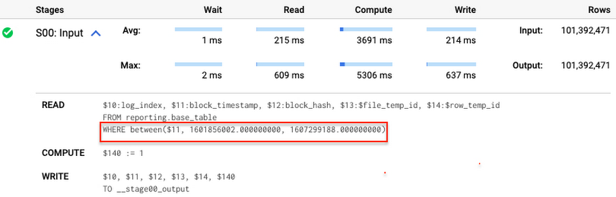
Note that you add the static filter to the staging table and keep T.block_timestamp = S.block_timestamp to convey to BigQuery that it can push that filter to the base table. This MERGE processes 41 GB of data in contrast to the initial 161 GB. You can see in the query plan that BigQuery pushes the partition filter from the staging table to the base table:
This type of optimization, when a pruning condition is pushed from a subquery to a large partitioned or clustered table, is not unique for MERGE. It also works for other types of queries. For instance:
SELECT * -- 41 GB processedFROM reporting.base_table TINNER JOIN staging.load_delta SON T.block_hash = S.block_hashAND T.log_index = S.log_indexAND T.block_timestamp = S.block_timestampWHERE S.block_timestamp BETWEEN TIMESTAMP '2020-10-05' AND TIMESTAMP '2020-12-07'
And you can check the query plan to verify that BigQuery pushed down the partition filter from one table to another.
Moreover, for SELECT statements, BigQuery can automatically infer a filter predicate on a join column and push it down from one table to another if your query meets the following criteria:
- The target table must be clustered or partitioned.
- The result size of the other table, i.e. after applying all filters, must qualify for broadcast join. Namly, the result set must be relatively small, less than ~100MB.
In our running example, reporting.base_table is partitioned by block_timestamp. If you define a selective filter on staging.load_delta and join two tables, you can see an inferred filter on the join key pushed to the target table
SELECT *FROM reporting.base_table TINNER JOIN staging.load_delta SON T.block_timestamp = S.block_timestampWHERE S.block_hash = '0x0c1caa16b34d94843aabfebc0d5a961db358135988f7498a6fdc450ad55f0870'
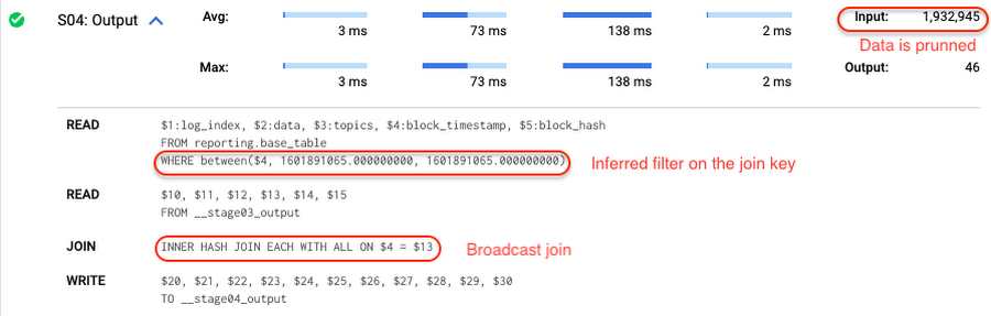
There is no requirement to join tables by partitioning or clustering key to kick off this type of optimization. However, in this case the pruning effect on the target table would be less significant.
But let us get back to the pipeline optimizations. Another way to enhance MERGE is to modify the merge_condition filter by adding static predicate on the base table:
BEGINDECLARE src_range STRUCT<date_min TIMESTAMP, date_max TIMESTAMP> --115 MB processedDEFAULT(SELECT STRUCT(MIN(block_timestamp) AS date_min,MAX(block_timestamp) AS date_max) FROM staging.load_delta);MERGE INTO reporting.base_table T --41 GB processedUSING staging.load_delta SON T.block_hash = S.block_hashAND T.log_index = S.log_indexAND T.block_timestamp BETWEEN src_range.date_min AND src_range.date_maxWHEN MATCHED THEN UPDATE SETT.data = S.dataWHEN NOT MATCHED THEN INSERT (log_index, data, topics, block_timestamp, block_hash)VALUES (log_index, data, topics, block_timestamp, block_hash);END;
To summarize, here are the steps that you can perform to enhance incremental ingestion pipelines in BigQuery. First you compute the range of updated partitions based on the small staging table. Next, you tweak the MERGE statement a bit to let BigQuery know to prune data in the base table.
All the enhanced MERGE statements scanned 41 GB of data, and setting up the src_range variable took 115 MB. Compare it with the initial 161 GB scan. Moreover, given that computing src_range may be incorporated into some existing transformation in your ETL/ELT, it results in a good performance improvement which you can leverage in your pipelines.
In this post we described how to enhance data ingestion pipelines by turning dynamic filter predicates into static predicates and letting BiQuery prune data for us. You can find more tips on BigQuery DML tuning here.
Special thanks to Daniel De Leo, who helped with examples and provided valuable feedback on this content.
A Look Back on Google Cloud’s Data Analytics Development Efforts from June

5984
Of your peers have already read this article.
4:00 Minutes
The most insightful time you'll spend today!
June is the month that holds the summer solstice, and some of us in the northern hemisphere get to enjoy the longest days of sunshine out of the entire year. We used all the hours we could in June to deliver a flurry of new features across BigQuery, Dataflow, Data Fusion, and more. Let’s take a look!
Simple, Sophisticated, and Secure
Usability is a key tenant of our data analytics development efforts. Our new user-friendly BigQuery improvements this month include:
- Flexible data type casting
- Formatting to change column descriptions
- GRANT/REVOKE access control commands using SQL
We hope this will delight data analysts, data scientists, DBAs, and SQL-enthusiasts who can find out more details in our blog here.
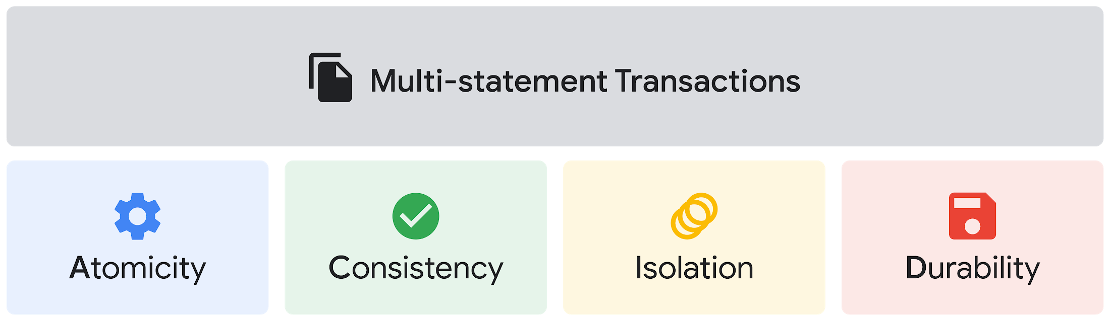
Beyond simplifying commands, we also recognize that it’s equally important to have more sophistication when dealing with transactions. That’s why we introduced multi-statement transactions in BigQuery.
As you probably know, BigQuery has long supported single-statement transactions through DML statements, such as INSERT, UPDATE, DELETE, MERGE and TRUNCATE, applied to one table per transaction. With multi-statement transactions, you can now use multiple SQL statements, including DML, spanning multiple tables in a single transaction.
This means that any data changes across multiple tables associated with all statements in a given transaction are committed atomically (all at once) if successful—or all rolled back atomically in the event of a failure.
We also know that organizations need to control access to data, down to the granular level and that, with the complexity of data platforms increasing day by day, it’s become even more critical to identify and monitor who has access to sensitive data.
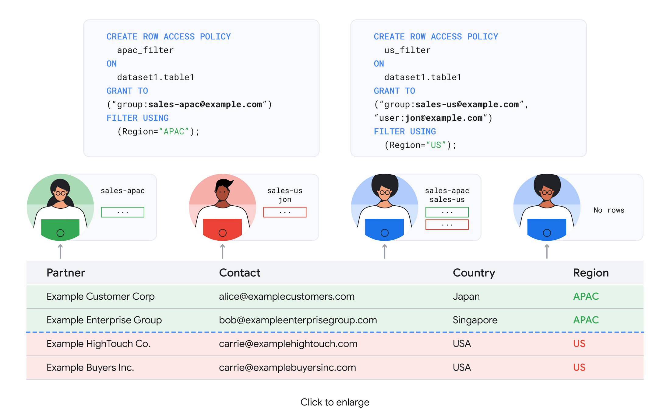
To help address these needs, we announced the general availability of BigQuery row-level security. This capability gives customers a way to control access to subsets of data in the same table for different groups of users. Row-level security in BigQuery enables different user personas access to subsets of data in the same table and can easily be created, updated, and dropped using DDL statements. To learn more, check out the documentation and best practices.
Simple, Safe, and Smart
Beyond building a simpler, more sophisticated and more secure data platform for customers, our team has been focused on providing solutions powered by built-in intelligence. One of our core beliefs is that for machine learning to be adopted and useful at scale, it must be easy to use and deploy.
BigQuery ML, our embedded machine learning capabilities, have been adopted by 80% of our top customers around the globe and it has become a cornerstone of their data to value journey.
As part of our efforts, we announced the general availability of AutoML tables in BigQuery ML. This no-code solution lets customers automatically build and deploy state-of-the-art machine learning models on structured data. With easy integration with Vertex AI, AutoML in BQML makes it simple to achieve machine learning magic in the background. From preprocessing data to feature engineering and model tuning all the way to cross validation, AutoML will “automagically” select and ensemble models so everyone—even non-data scientists—can use it.
Want to take this feature for a test drive? Try it today on BigQuery’s NYC Taxi public dataset following the instructions in this blog!
Speaking of public datasets, we also introduced the availability of Google Trends data in BigQuery to enable customers to measure interest in a topic or search term across Google Search. This new dataset will soon be available in Analytics Hub and will be anonymized, indexed, normalized, and aggregated prior to publication.
Want to ensure your end-cap displays are relevant to your local audience? You can take signals from what people are looking for in your market area to inform what items to place. Want to understand what new features could be incorporated into an existing product based on what people are searching for? Terms that appear in these datasets could be an indicator of what you should be paying attention to.
All this data and technology can be put to use to deploy critical solutions to grow and protect your business. For example, it can be difficult to know how to define anomalies during detection. If you have labeled data with known anomalies, then you can choose from a variety of supervised machine learning model types that are already supported in BigQuery ML.
But what if you don’t know what kind of anomaly to expect, and you don’t have labeled data? Unlike typical predictive techniques that leverage supervised learning, organizations may need to be able to detect anomalies in the absence of labeled data.
That’s why, we were particularly excited to announce the public preview of new anomaly detection capabilities in BigQuery ML that leverage unsupervised machine learning to help you detect anomalies without needing labeled data.
Our team has been working with a large number of enterprises who leverage machine learning for better anomaly detection. In financial services for example, customers have used our technology to detect machine-learned anomalies in real-time foreign exchange data.
To make it easier for you to take advantage of their best practices, we teamed up with Kasna to develop sample code, architecture guidance, and a data synthesizer that generates data so you can test these innovations right away.
Simple, Scalable, and Speedy
Capturing, processing and analyzing data in motion has become an important component of our customer architecture choices. Along with batch processing, many of you need the flexibility to stream records into BigQuery so they can become available for query as they are written.
Our new BigQuery Storage Write API combines the functionality of streaming ingestion and batch loading into a single API. You can use it to stream records into BigQuery or even batch process an arbitrarily large number of records and commit them in a single atomic operation.
Flexible systems that can do batch and real-time in the same environment is in our DNA: Dataflow, our serverless, data processing service for streaming and batch data was built with flexibility in mind.
This principle applies not just to what Dataflow does but also how you can leverage it—whether you prefer using Dataflow SQL right from the BigQuery web UI, Vertex AI notebooks from the Dataflow interface, or the vast collection of pre-built templates to develop streaming pipelines.
Dataflow has been in the news quite a bit recently. You might have noted the recent introduction of Dataflow Prime, a new no-ops, auto-tuning functionality that optimizes resource utilization and further simplifies big data processing. You might have also read that Google Dataflow is a Leader in The 2021 Forrester Wave™: Streaming Analytics, giving Dataflow a score of 5 out of 5 across 12 different criteria.
We couldn’t be more excited about the support the community has provided to this platform. The scalability of Dataflow is unparalleled and as you set your company up for more scale, more speed, and “streaming that screams”, we suggest you take a look at what leaders at Sky, RVU or Palo Alto Networks have already accomplished.
If you’re new to Dataflow, you’re in for a treat: this past month, Priyanka Vergadia (AKA CloudGirl) released a great set of resources to get you started. Read her blog here and watch her introduction video below!
https://youtube.com/watch?v=WRspZRG9e90%3Fenablejsapi%3D1%26
Simple structure that sticks together
We thrive to be the partner of choice for your transformation journey, regardless where your data comes from and how you choose to unify your data stack.
Our partners at Tata Consultancy Services (TCS) recently released research that highlights the importance of a unifying digital fabric and how data integration services like Google Cloud Data Fusion can enable their clients to achieve this vision.
We also announced SAP Integration with Cloud Data Fusion, Google Cloud’s native data integration platform, to seamlessly move data out of SAP Business Suite, SAP ERP and S4/HANA. To date, we provide more than 50 pipelines in Cloud Data Fusion to rapidly onboard SAP data.
This past month, we introduced our SAP Accelerator for Order to Cash. This accelerator is a sample implementation of the SAP Table Batch Source feature in Cloud Data Fusion and will help you get started with your end-to-end order to cash process and analytics.
It includes sample Cloud Data Fusion pipelines that you can configure to connect to your SAP data source, perform transformations, store data in BigQuery, and set up analytics in Looker. It also comes with LookML dashboards which you can access on Github.
Countless great organizations have chosen to work with Google for their SAP data. In June, we wrote about ATB Financial’s journey and how the company uses data to better serve over 800,000 customers, save over CA$2.24 million in productivity, and realize more than CA$4 million in operating revenue through “D.E.E.P”, a data exposure enablement platform built around BigQuery.
Finally, if you are an application developer looking for a unified platform that brings together data from Firebase Crashlytics, Google Analytics, Cloud Firestore, and third party datasets, we have good news!
This past month, we released a unified analytics platform that combines Firebase, BigQuery, Google Looker and FiveTran to easily integrate disparate data sources, and infuse data into operational workflows for greater product development insights and increased customer experience. This resource comes with sample code, a reference guide and a great blog! We hope you enjoy it. See you all next month!
https://youtube.com/watch?v=L25Vfzr2Ciw%3Fenablejsapi%3D1%26
How Google Cloud Solutions Help Retail Firms to ABP(Always Be Pivoting)

6418
Of your peers have already read this article.
2:00 Minutes
The most insightful time you'll spend today!
For years, retailers have been told that they must embrace a litany of new technologies, trends, and imperatives like online shopping, mobile apps, omnichannel, and digital transformation. In search of growth and stability, retailers adopted many of these, only to realize that for every box they ticked, there was another one waiting.
And then the pandemic hit, along with rising social movements and increasingly harsh weather. Some retailers were more prepared to take on these disruptions than others, which crystallized a new universal truth across the industry: the ability to adapt on the fly became the most important trait to survive and thrive.
Today’s retail landscape has surfaced both existing and new challenges for specialty and department store retailers. Approximately 88% of purchases previously occurred within a store environment. Now, it’s closer to 59%, with the remainder done online or through other omni methods.
With such constant change and upheaval, it can feel like the mantra now is ABP: always be pivoting.
The big question isn’t just how to maintain constant momentum and agility—it’s how to do it without sapping your workforce, your inventory, or your profits in the process. The pivot is now a given. What matters is how you do it.
Adapting requires a flexible base of technology that allows retailers to shift and scale seamlessly with the needs of the moment.
They need to be able to leverage real-time insights and enhance customer experiences rapidly, online and in the real world (not to mention the growing hybridization that’s AR and VR). They need to modernize their stores to power engaging consumer and associate experiences. They need to enhance operations for rapid scaling between full operations and digital-only offerings.
To help retailers achieve these goals and more, Google Cloud is honing a trio of essential innovations: demand forecasting that harnesses the power of data analytics and artificial intelligence; enhanced product discovery to improve conversion across channels; and the tools to help create the modern store experience.
In other words, here’s some of the biggest ways we’re ready to help you pivot.
Pivot point 1: Harnessing data and AI for demand forecasting with Vertex AI
One of the greatest challenges for retailers when building organizational flexibility is managing inventory and the supply chain.
We are in the midst of one of the worst global supply chain crises, stemming from soaring demand and logistics issues brought on by the pandemic. This crisis has only heightened the challenge retailers face when assessing demand and product availability. Even in normal times, mismanagement of inventory can add up to a trillion-dollar problem, according to IHL Group (costing $634 billion in lost sales worldwide each year, while overstocks result in $472 billion in lost revenues due to markdowns).
On the flipside, optimizing your supply chain can lead to greater profits. For instance, McKinsey predicts that a 10% to 20% improvement in retail supply chain forecasting accuracy is likely to produce a 5% reduction in inventory costs and a 2% to 3% increase in revenues.
Some of the challenges related to demand forecasting include:
- Low accuracy leads to excess inventory, missed sales, and pressure on fragile supply chains.
- Real drivers of product demand are not included, because large datasets are hard to model using traditional methods.
- Poor accuracy for new product launches and products that have sparse or intermittent demand.
- Complex models are hard to understand, leading to poor product allocation and low return on investment on promotions.
- Different departments use different methods, leading to miscommunication and costly reconciliation errors.
AI-based demand forecasting techniques can help. Vertex AI Forecast supports retailers in maintaining greater inventory flexibility by infusing machine learning into their existing systems. Machine learning and AI-based forecasting models like Vertex AI are able to digest large sets of disparate data, drive analytics and automatically adjust when provided with new information.
With these machine learning models, retailers can not only incorporate historical sales data, but also use close to real-time data such as marketing campaigns, web actions like a customer clicking the “add to cart” button on a website, local weather forecasts, and much more.
Pivot point 2: Enhanced product discovery through AI-powered search and recommendations
If customers can’t easily find what they are looking for, whether online or at the store, they will turn to someone else. That’s a simple statement, but one with profound impacts.
In research conducted by The Harris Poll and Google Cloud, we found that over a six month period, 95% of consumers received search results that were not relevant to what they were searching for on a retail website. And roughly 85% of consumers view a brand differently after an unsuccessful search, while 74% say they avoid websites where they’ve experienced search difficulties in the past.
Each year, retailers lose more than $300 billion dollars from search abandonment, or when a consumer searches for a product on a retailer’s website but does not find what they are looking for. Our product discovery solutions help you surface the right products, to the right customers, at the right time. These solutions include:
- Vision Product Search, which is like bringing the augmented reality of Google Lens to a retailer’s own branded mobile app experience. Both shoppers and retail store associates can search for products using an image they’ve photographed or found online and receive a ranked list of similar items.
- Recommendations AI, which enables retailers to deliver highly personalized recommendations at scale across channels.
- Retail Search, which provides Google-quality search results on a retailer’s own website and mobile applications.
All three are powered by Google Cloud, leveraging Google’s advanced understanding of user context and intent, utilizing technology to deliver a seamless experience to every shopper. With these combined capabilities, retailers are able to reduce search abandonment and improve conversions across their digital properties.
Pivot point 3: Building the modern store
Stores are no longer places for just browsing and buying. They must be flexible operation centers, ready to pivot to address changing circumstances. The modern store must be multiple things at once: a mini-fulfillment and return center, a recommendation engine, a shopping destination, a fun place to work, and more.
Just as retail companies had to embrace omnichannel, stores are now becoming omnichannel centers on their own, mixing the digital and physical into a single location. Retailers can use physical stores as a vehicle to deliver superior customer experiences. This will demand heightened levels of collaboration and cooperation between stores, digital, and tech infrastructure teams, building on the agile ways they have worked together.
In many ways, it’s about allowing our physical spaces to function more like digital ones. Google Cloud can help by bringing the scalability, security, and reliability of the cloud to the store, allowing physical locations to upgrade infrastructure and modernize their internal and customer-facing applications.
Think of it as when a new OS gets released for your phone. It’s the same small, hard box, but the experience can feel radically different. Now, extend that same idea to a digitally enabled store. With the right displays, interfaces, and tools at a given retail location, the team only needs to send an over-the-air update to create radically fresh experiences, ranging from sales displays to fulfillment or employee engagement.
Such an approach can enable streamlined experiences for both customers and store associates. For instance, when it comes to the modern store’s evolving role as a fulfillment or return center, cloud solutions can help drive efficiency in stores through automation of ordering, replenishment, and fulfillment of omnichannel order selection.
Similar tools for personalized product discovery online can be applied to customers in the store, helping them to browse and explore, or even create a tailored shopping experience.
The impact of store associates can be maximized by equipping them with technology to provide expertise that drives value-added customer service, as well as increasing productivity in stores by streamlining operations, thus lowering overhead cost. At the register, customers should be able to enjoy frictionless checkout while ensuring reliable, accurate, secure transactions.
Google Cloud can help retailers transform
The ability to adapt and pivot to meet today’s changing consumer needs requires that retailers rely on modern tools to obtain operational flexibility. We believe that every company can be a tech company. That every decision is data driven. That every store is physical and digital all at once. That every worker is a tech worker.
Google Cloud works with retailers to help them solve their most challenging problems. We have the unique ability to handle massive amounts of unstructured data, in addition to advanced capabilities in AI and ML. Our products and solutions help retailers focus on what’s most important—from improving operations to capturing digital and omnichannel revenue.
STAC-M3 Tick History Analytics in Google Cloud Benchmark Results Reveals it is 18X Faster than Previous Version

4772
Of your peers have already read this article.
5:00 Minutes
The most insightful time you'll spend today!
The Securities Technology Analysis Center (STAC®), an organization that improves technology discovery and assessment in the finance industry through dialog and research, recently audited the STAC-M3™ benchmark suite on Google Cloud (SUT ID KDB211210). These enterprise tick-analytics benchmarks assess the ability of a solution stack such as database software, servers, and storage, to perform a variety of I/O-intensive and compute-intensive operations on historical market data.
Following up on our previous STAC-M3 benchmark audit (SUT ID KDB181001), a redesigned Google Cloud architecture leveraged the most recent version of kdb+ 4.0, the time-series database from KX, and achieved significant improvements: 35 out of 41 benchmarks ran faster in the new cluster – by up to 18x faster than Google Cloud’s prior results. Key highlights include the following:
Compared to the previous STAC-M3 Antuco suite results on Google Cloud:
- Was faster in 13 of 17 mean response-time benchmarks
- Was 18x faster – a 94% reduction in run time – in the version of Year-High Bid that allows caching (STAC-M3.ß1.1T.YRHIBID-2.TIME), which also set an overall record for all published results
- Had 9x higher throughput in Year-High Bid (STAC-M3.ß1.1T.YRHIBID.MBPS)
Compared to the previous STAC-M3 Kanaga suite results on Google Cloud:
- Was faster in 22 of 24 mean response-time benchmarks
- Was over 10x faster in all four Market Snapshot workloads (STAC-M3.ß1.10T.YR[2,3,4,5]-MKTSNAP.TIME)
- Had 5x the throughput in Year-High Bid involving 2 years of data (STAC-M3.ß1.1T.2YRHIBID.MBPS)
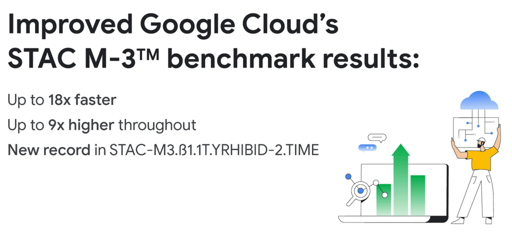
“The STAC-M3 standard was designed by financial firms to reveal the performance of tick analytics stacks. Generational improvements like those exhibited by Google Cloud’s most recent STAC-M3 audit, are important data points for firms evaluating new architectures for performance and scale,” said Peter Nabicht, President of STAC.
These performance results may translate to real-world advantages that may be difficult for investment firms to achieve in static and costly on-premises environments: immediate answers in high data velocity markets, more thoroughly explored research theories by adding data or new quantitative approaches, and reduced costs by releasing cloud resources more quickly.
STAC-M3: High-speed tick analytics
Designing for record-breaking results
In our STAC-M3 audit, the stack under test (SUT) was designed to take advantage of horizontal scalability in the cloud by sharding data across independent compute nodes. The cluster of 12 Google Compute Engine N2 instances was powered by Intel Cascade Lake, with each node using 32 vCPUs, 160GiB of memory, and 9TiB of local NVMe SSDs. The full STAC-M3 Antuco and Kanaga data set was split across the cluster and kdb+ scripts distributed queries between nodes.
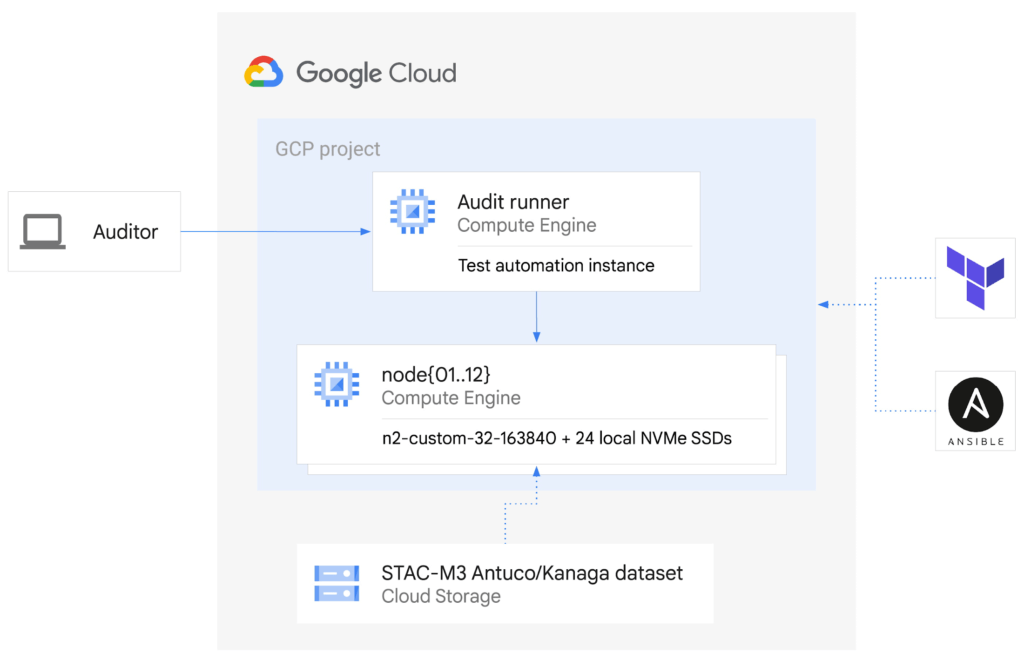
This configuration was the sweet spot for this particular workload, but this architecture does not need to be limited to 12 nodes for other workloads – the data sharding algorithm could scale to any number of nodes as required by workload demands. Since scaling out the cluster in this manner increases the total pool of available storage, this architecture can continue scaling out to petabytes of storage across hundreds of nodes.
The ability to spawn large clusters with hundreds of thousands of processors on demand at low cost, and to delete the resources when jobs complete, not only changes the economics of running computations on large financial data sets, it also opens up opportunities to explore solutions to new types of problems that were previously overlooked due to the constraints of fixed hardware on-premises. You can check the pricing of this VM configuration using the Google Cloud Pricing Calculator. The costs can be reduced even further by using preemptible VMs.
While the new cluster used a similar number of nodes, cores, and total memory as the previously-audited cluster, the redesigned architecture allowed us to harness the low latency and high throughput of Local NVMe SSDs.
Resources on demand
The cluster was created on demand using Terraform and Ansible during testing and auditing. The use of infrastructure as code (IaC) techniques ensured that the cluster, fully loaded with the STAC-M3 data set, could be created when needed and then removed when benchmarking was complete. It also meant that the cluster configuration was enforced by code on each deployment, eliminating configuration variance and drift. The full IaC definition to create the cluster can be retrieved from the report in the STAC Vault.
Each time the cluster was created, data was streamed to Local SSDs from Google Cloud Storage, our reliable and secure object storage, at up to the line rate of 32Gbps per node. The entire 57TiB STAC-M3 Antuco and Kanaga data was replicated from Cloud Storage to local storage in approximately 20 minutes.
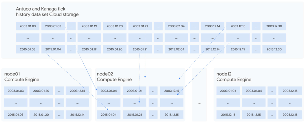
Since each node was independent and responsible for its own shard of data, doubling the cluster size would cut the synchronization time in half, or copy twice as much data in the same amount of time. Using higher bandwidth options of up to 100Gbps would triple the possible throughput for a relatively small incremental cost, trading an approximately 11%-23% price increase at current list prices for a 200% data synchronization performance increase. Taking advantage of fast networking to cache sharded data in parallel to a large cluster makes storing bulk data in Cloud Storage viable for even the largest workloads.
For quants working on vast data sets in sprawling compute clusters, the ability to fully describe infrastructure as declarative code, create elastic resources on demand, cache data quickly from cheap bulk storage, and turn resources off when computations complete is a dramatic change compared to waiting months to grow on-premises clusters – and a compelling reason to use cloud infrastructure.
To see how we designed and optimized the cluster for API-driven cloud resources, read our new whitepaper.
STAC-A2™: Calculating derivatives risk
In 2018, we showed that cloud instances can outperform bare metal when analyzing large tick history data sets in the demanding suite of STAC-M3 benchmarks. Last year, Google Cloud’s partner Appsbroker showed that the same was true for calculating derivatives risk in STAC-A2 on Google Cloud. You can read about how Appsbroker built its record-breaking STAC-A2 compute cluster on Google Cloud in its blog post, or access the STAC Report directly. Here are the highlights:
Compared to all other publicly reported solutions, this solution, based on a cluster of 10 virtual machines, had:
- The highest throughput (STAC-A2.β2.HPORTFOLIO.SPEED)
- The fastest cold time in the large problem size (STAC-A2.β2.GREEKS.10-100k-1260.TIME.COLD)
Compared to a solution involving an 8-node, on-premises cluster (SUT ID INTC181012), this 10-node, cloud-based solution:
- Had 5 times the maximum paths (STAC-A2.β2.GREEKS.MAX_PATHS)
- Had 10% greater throughput (STAC-A2.β2.HPORTFOLIO.SPEED)
- Was 18% faster in cold runs of the large problem size (STAC-A2.β2.GREEKS.10-100k-1260.TIME)
- Was 9% faster in cold runs of the baseline problem size (STAC-A2.β2.GREEKS.TIME.COLD)
Finding market advantages with Google Cloud
Across the investment management industry, every firm is seeking many of the same competitive advantages. However, finding unique opportunities and managing larger and larger data sets is becoming a major strain. Cloud is fundamentally changing how quants tackle the problem while empowering them to manage risk and generate higher returns.
Building on-premises computing clusters with tens or hundreds of thousands of cores and petabytes of storage requires huge up-front investments and lead time measured in months or years. Google Cloud makes the same scale available to its customers, provisioned on demand and paid per use. More importantly, the elasticity of cloud resources enables agility that is simply not available in a fixed data center cluster – the agility to explore, experiment, iterate, and respond to markets faster than before.
Scaling out to tens of thousands of cores in minutes and then removing the resources immediately not only changes the speed at which questions can be answered; it encourages different and more frequent questions, asked simultaneously on many independent clusters, free from the constraints of fixed on-premises hardware.
It is this flexibility and power that enables financial services firms to leverage larger data sets and get results, backtest, research, and analyze large amounts of data, faster and whenever they need it.
Download our whitepaper to learn more about our latest STAC-M3 tick history analytics benchmark results and how to optimize cloud infrastructure for high-speed market data analysis.
More Relevant Stories for Your Company



What’s New in BigQuery, Google Cloud’s Modern Data Warehouse
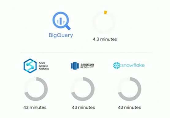
The demands that today's enterprise has from data go far beyond the capabilities of traditional data warehousing. For many leaders, the need to digitally transform their businesses is a key driver for data analytics spending. Businesses want to make real-time decisions from fresh information as well as make predictions from



Google had Enough of Flooding in India. Here’s What It Did About It
Over the last century, floods have become the most common and deadly natural disaster on the planet. Many countries currently lack effective early warning systems and alerts. Today, 20 percent of flood fatalities occur in India. To help, Google sent a team to study the Ghaghara River, near Patna. “In

Cart.com to Transform e-Commerce for Brands Globally
The ecommerce playing field has been hard to navigate for most retailers, and Cart.com is on a mission to change that. Traditionally, retailers needing to run their online store, order fulfillment, customer service, marketing, and other essential activities have had to cobble together systems to get the capabilities they need

A Comprehensive Guide for Understanding and Optimizing Your Dataflow Costs
Dataflow is the industry-leading platform that provides unified batch and streaming data processing capabilities, and supports a wide variety of analytics and machine learning use cases. It’s a fully managed service that comes with flexible development options (from Flex Templates and Notebooks to Apache Beam SDKs for Java, Python and Go),
