





Leverage ML to Spot Anomalies in Real-time Forex Data

3109
Of your peers have already read this article.
6:00 Minutes
The most insightful time you'll spend today!
Let’s say you are a quantitative trader with access to real-time foreign exchange (forex) price data from your favorite market data provider. Perhaps you have a data partner subscription, or you’re using a synthetic data generator to prove value first. You know there must be thousands of other quants out there with your same goal. How will you differentiate your anomaly detector?
What if, instead of training an anomaly detector on raw forex price data, you detected anomalies in an indicator that already provides generally agreed buy and sell signals? Relative Strength Index (RSI) is one such indicator; it is often said that RSI going above 70 is a sell signal, and RSI going below 30 is a buy signal. As this is just a simplified rule, it means there could be times when the signal is inaccurate, such as a currency market correction, making it a prime opportunity for an anomaly detector.
This gives us the following high level components:

Of course, we want each of these components to handle data in real time, and scale elastically as needed. Dataflow pipelines and Pub/Sub are the perfect services for this. All we need to do is write our components on top of the Apache Beam sdk, and they’ll have the benefit of distributed, resilient and scalable compute.
Luckily for us, there are some great existing Google plugins for Apache Beam. Namely, a Dataflow time-series sample library that includes RSI calculations, and a lot of other useful time series metrics; and a connector for using AI Platform or Vertex AI inference within a Dataflow pipeline. Let’s update our diagram to match, where the solid arrows represent Pub/Sub topics.
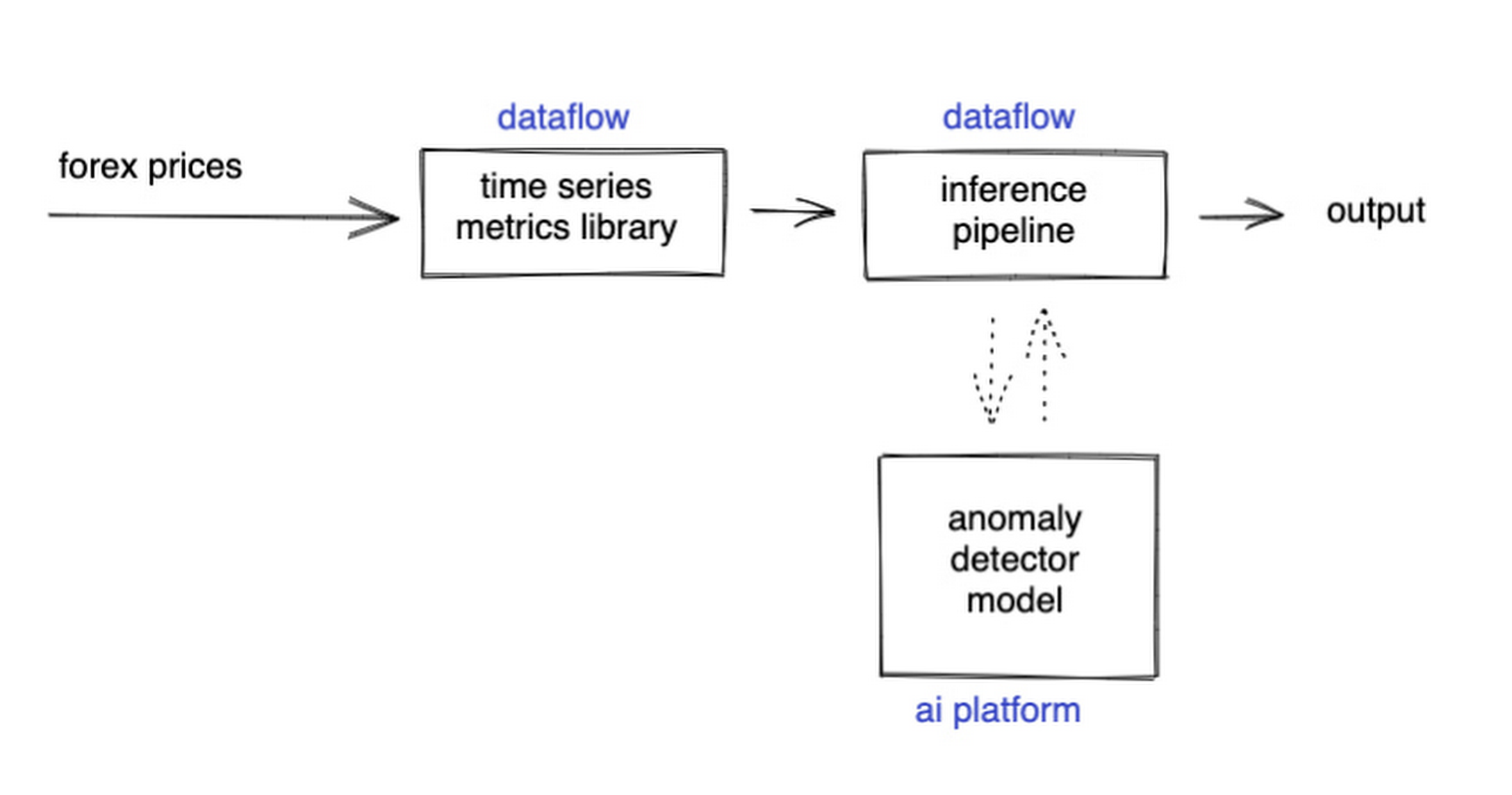
The Dataflow time-series sample library also provides us with gap-filling capabilities, which means we can rely on having contiguous data once the flow reaches our machine learning (ML) model. This lets us implement quite complex ML models, and means we have one less edge case to worry about.
So far we’ve only talked about the real time data flow, but for visualization and continuous retraining of our ML model, we’re going to want historical data as well. Let’s use BigQuery as our data warehouse, and Dataflow to plumb Pub/Sub into it. As this plumbing job is embarrassingly parallelizable, we wrote our pipeline to be generic across data types and share the same Dataflow job, such that compute resources can be shared. This results in efficiencies of scale both in cost savings and time required to scale-up.

Data Modeling
Let’s discuss data formats a bit further here. An important aspect of running any data engineering project at scale is flexibility, interoperability and ease of debugging. As such, we opted to use flat JSON structures for each of our data types, because they are human readable and ubiquitously understood by tooling. As BigQuery understands them too, it’s easy to jump into the BigQuery console and confirm each component of the project is working as expected.
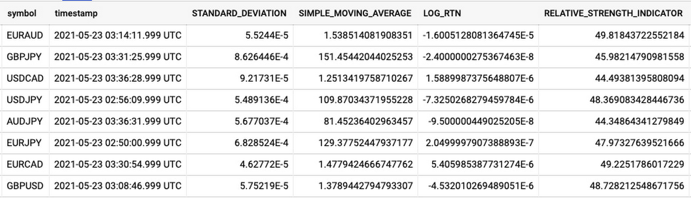
As you can see, the Dataflow sample library is able to generate many more metrics than RSI. It supports generating two types of metrics across time series windows, metrics which can be calculated on unordered windows, and metrics which require ordered windows, which the library refers to as Type 1 metrics and Type 2 metrics, respectively. Unordered metrics have a many-to-one relationship, which can help reduce the size of your data by reducing the frequency of points through time. Ordered metrics run on the outputs of the unordered metrics, and help to spread information through the time domain without loss in resolution. Be sure to check out the Dataflow sample library documentation for a comprehensive list of metrics supported out of the box.
As our output is going to be interpreted by our human quant, let’s use the unordered metrics to reduce the time resolution of our flow of real time data to one per second, or one hertz. If our output was being passed into an automated trading algorithm, we might choose a higher frequency. The decision for the size of our ordered metrics window is a little more difficult, but broadly determines the amount of time-steps our ML model will have for context, and therefore the window of time for which our anomaly detection will be relevant. We at least need it to be larger than our end-to-end latency, to ensure our quant will have time to act. Let’s set it to five minutes.
Data Visualization
Before we dive into our ML model, let’s work on visualization to give us a more intuitive feel for what’s happening with the metrics, and confirm everything we’ve got so far is working. We use the Grafana helm chart with the BigQuery plugin on a Google Kubernetes Engine (GKE) Autopilot cluster. The visualisation setup is entirely config-driven and provides out-of-the-box scaling, and GKE gives us a place to host some other components later on.
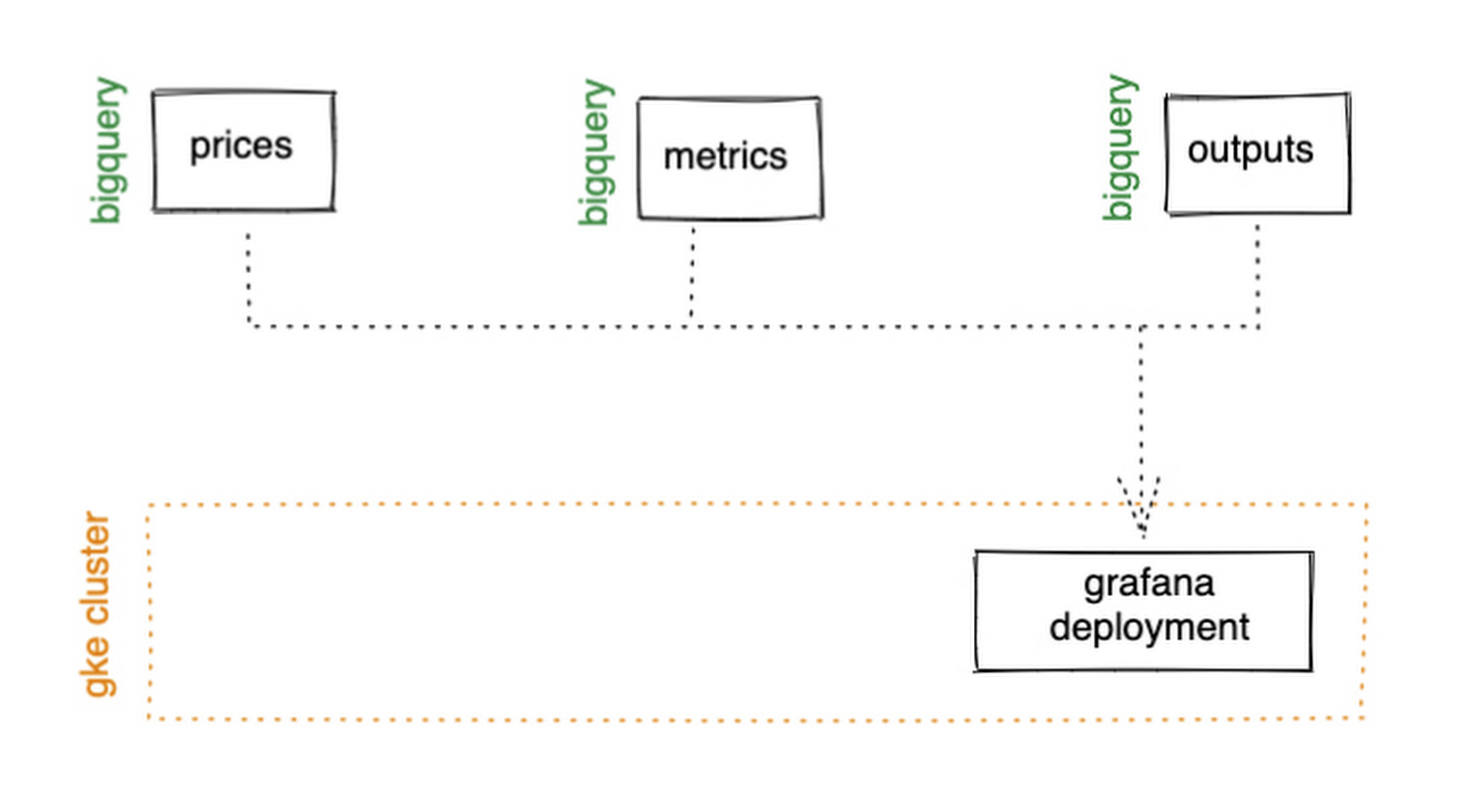
GKE Autopilot has Workload Identity enabled by default, which means we don’t need to worry about passing around secrets for BigQuery access, and can instead just create a GCP service account that has read access to BigQuery and assign it to our deployment through the linked Kubernetes service account.
That’s it! We can now create some panels in a Grafana dashboard and see the gap filling and metrics working in real time.

Building and deploying the Machine Learning Model
Ok, ML time. As we alluded to earlier, we want to continuously retrain our ML model as new data becomes available, to ensure it remains up to date with the current trend of the market. TensorFlow Extended (TFX) is a platform for creating end-to-end machine learning pipelines in production, and eases the process around building a reusable training pipeline. It also has extensions for publishing to AI Platform or Vertex AI, and it can use Dataflow runners, which makes it a good fit for our architecture. The TFX pipeline still needs an orchestrator, so we can host that in a Kubernetes job, and if we wrap it in a scheduled job, then our retraining happens on a schedule too!

TFX requires our data be in the tf.Example format. The Dataflow sample library can output tf.Examples directly, but this tightly couples our two pipelines together. If we want to be able to run multiple ML models in parallel, or train new models on existing historical data, we need our pipelines to only be loosely coupled. Another option is to use the default TFX BigQuery adaptor, but this restricts us to each row in BigQuery mapping to exactly one ML sample, meaning we can’t use recurrent networks.
As neither of the out-of-the-box solutions met our requirements, we decided to write a custom TFX component that did what we needed. Our custom TFX BigQuery adaptor enables us to keep our standard JSON data format in BigQuery and train recurrent networks, and it keeps our pipelines loosely coupled! We need the windowing logic to be the same for both training and inference time, so we built our custom TFX component using standard Beam components, such that the same code can be imported in both pipelines.
def window_elements(pipeline: beam.Pipeline,window_length: int,drop_irregular_windows: bool = True,sort_windows_by: str = "timestamp",):"""Window elements into regular windows of a given size.Assumes elements flow at a fixed rate of 1Hz."""def _sort_windows(window: Iterable[Dict[Text, Any]]) -> List[Dict[Text, Any]]:sorted_window = sorted(window, key=lambda e: e[sort_windows_by])return sorted_windowwindowed_elements = (pipeline| "AddConstantKey" >> beam.Map(lambda item: (0, item))| "WithSlidingWindow">> beam.WindowInto(beam.transforms.window.SlidingWindows(window_length, 1),trigger=beam.transforms.trigger.AfterCount(window_length),accumulation_mode=beam.transforms.trigger.AccumulationMode.DISCARDING,)| "CombineWindow" >> beam.GroupByKey()| "GetValues" >> beam.Values())if drop_irregular_windows:windowed_elements = windowed_elements | "EnforceWindowLengths" >> beam.Filter(lambda w: len(w) == window_length).with_output_types(List[Dict[Text, Any]])if sort_windows_by is not None:windowed_elements = windowed_elements | "Sort" >> beam.Map(_sort_windows).with_output_types(List[Dict[Text, Any]])return windowed_elements
With our custom generator done, we can start designing our anomaly detection model. An autoencoder utilising long-short-term-memory (LSTM) is a good fit for our time-series use case. The autoencoder will try to reconstruct the sample input data, and we can then measure how close it gets. That difference is known as the reconstruction error. If there is a large enough error, we call that sample an anomaly. To learn more about autoencoders, please consider reading chapter 14 from Deep Learning by Ian Goodfellow, Yoshua Bengio, and Aaron Courville.
Our model uses simple moving average, exponential moving average, standard deviation, and log returns as input and output features. For both the encoder and decoder subnetworks, we have 2 layers of 30 time step LSTMs, with 32 and 16 neurons, respectively.
In our training pipeline, we include z score scaling as a preprocessing transformer – which is usually a good idea when it comes to ML. However, there’s a nuance to using an autoencoder for anomaly detection. We need not only the output of the model, but also the input, in order to calculate the reconstruction error. We’re able to do this by using model serving functions to ensure our model returns both the output and preprocessed input as part of its response. As TFX has out-of-the-box support for pushing trained models to AI Platform, all we need to do is configure the pusher, and our (re)training component is complete.
Detecting Anomalies in real time
Now that we have our model in Google Cloud AI Platform, we need our inference pipeline to call to it in real time. As our data is using standard JSON, we can easily apply our RSI rule of thumb inline, ensuring our model only runs when needed. Using the reconstructed output from AI Platform, we are then able to calculate the reconstruction error. We choose to stream this directly into Pub/Sub to enable us to dynamically apply an anomaly threshold when visualising, but if you had a static threshold you could apply it here too.
with beam.Pipeline(options=pipeline_options) as pipeline:(pipeline| "ReadFromPubSub">> beam.io.ReadFromPubSub(topic=input_metrics,timestamp_attribute=timestamp_key,)| "DeserialiseJSON" >> beam.Map(pubsub_serialiser.to_json)| "FilterSymbol" >> beam.Filter(lambda m: m["symbol"] == symbol)| "FilterRSIThreshold">> beam.Filter(lambda m: m["RELATIVE_STRENGTH_INDICATOR"] > rsi_upper_thresholdor m["RELATIVE_STRENGTH_INDICATOR"] < rsi_lower_threshold)| "WindowElements" >> window_elements(window_length)| "RunAutoencoder">> run_windowed_inference(gcp_project_id,model_name,window_length,{f: "FLOAT" for f in feature_metrics},)| "CalcReconError" >> beam.Map(calc_reconstruction_err)| "ToJSON">> beam.Map(lambda re: {"symbol": symbol, "reconstruction_error": re})| "SerialiseJSON" >> beam.Map(pubsub_serialiser.from_json)| "WriteToPubSub">> beam.io.WriteToPubSub(topic=output_alerts,timestamp_attribute=timestamp_key,))
Summary
Here’s what the wider architecture looks like now:

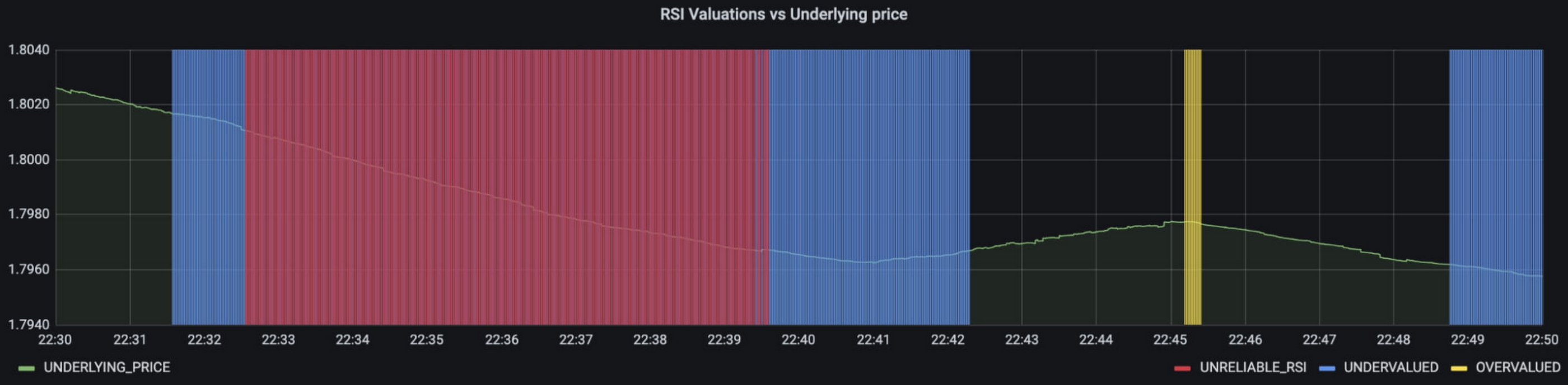
More importantly though, does it fit for our use case? We can plot the reconstruction error of our anomaly detector against the standard RSI buy/sell signal, and see when our model is telling us that perhaps we shouldn’t blindly trust our rule of thumb. Go get ‘em, quant!
In terms of next steps, there are many things you could do to extend or adapt what we’ve covered. You might want to explore with multi-currency models, where you could detect when the price action of correlated currencies is unexpected, or you could connect all of the Pub/Sub topics to a visualization tool to provide a real-time dashboard.
Give it a try
To finish it all off, and to enable you to clone the repo and set everything up in your own environment, we include a data synthesizer to generate forex data without needing access to a real exchange. As you might have guessed, we host this on our GKE cluster as well. There are a lot of other moving parts – TFX uses a SQL database and all of the application code is packaged into a docker image and deployed along with the infra using Terraform and cloud build. But if you’re interested in those nitty gritty details, head over to the repo and get cloning!
Feel free to reach out to our teams at Google Cloud and Kasna for help in making this pattern work best for your company.
Master AI Prompt Engineering with 6 Proven Tips

1056
Of your peers have already read this article.
2:30 Minutes
The most insightful time you'll spend today!
As AI-powered tools become increasingly prevalent, prompt engineering is becoming a skill that developers need to master. Large language models (LLMs) and other generative foundation models require contextual, specific, and tailored natural language instructions to generate the desired output. This means that developers need to write prompts that are clear, concise, and informative.
In this blog, we will explore six best practices that will make you a more efficient prompt engineer. By following our advice, you can begin creating more personalized, accurate, and contextually aware applications. So let’s get started!
Tip #1: Know the model’s strengths and weaknesses
As AI models evolve and become more complex, it is essential for developers to comprehend their capabilities and limitations. Understanding these strengths and weaknesses can help you, as a developer, avoid making mistakes and create safer, more reliable applications.
For example, an AI model that is trained to recognize images of blueberries may not be able to recognize images of strawberries. Why? Because the model was only trained on a dataset of blueberry images. If a developer uses this model to build an application that is supposed to recognize both blueberries and strawberries, the application would likely make mistakes, leading to an ineffective outcome, and poor user experience.
It’s important to note that AI models have the ability to be biased. This is due to AI models being trained on data that is collected from the real world, and so it can reflect the inequitable power dynamics inherently rooted in our social hierarchy. If the data that is used to train an AI model is biased, then the model will also be biased. This can lead to problems if the model is used to make decisions that affect people by reinforcing societal biases. Addressing these biases is important to ensure that data is fair, promoting equality, and ensuring the responsibility of AI technology. Prompt engineers should be aware of training limitations or biases so they can craft prompts more effectively and understand what kind of prompting is even possible for a given model.

Tip #2: Be as specific as possible
AI models have the ability to comprehend a variety of prompts. For instance Google’s PaLM 2 can understand natural language prompts, multilingual text, and even programming codes like Python and JavaScript. Although AI models can be very knowledgeable, they are still imperfect, and have the ability to misinterpret prompts that are not specific enough. In order for AI models to navigate ambiguity, it is important to tailor your prompts specifically to your desired outcome.
Let’s say you would like your AI model to generate a recipe for 50 vegan blueberry muffins. If you prompt the model with “what is a recipe for blueberry muffins?”, the model does not know that you need to make 50 muffins. It is thus unlikely to list the larger volume of ingredients you’ll need or include tips to help you more efficiently bake such a large number of muffins. The model can only go off the context that is provided. A more effective prompt would be “I am hosting 50 guests. Generate a recipe for 50 blueberry muffins.” The model is more likely to generate a response that is relevant to your request and meets your specific requirements.
Tip #3: Utilize contextual prompts
Utilize contextual information in your prompts to help the model gain an in-depth understanding of your requests. Contextual prompts can include the specific task you want the model to perform, a replica of the output you’re looking for, or a persona to emulate, from a marketer or engineer to a high school teacher. Defining a tone and perspective for an AI model gives it a blueprint of the tone, style, and focused expertise you’re looking for to improve the quality, relevance, and effectiveness of your output.
In the case of the blueberry muffins, it is important to prompt the model using the context of the situation. The model might need more context than generating a recipe for 50 people. If it needs to be aware that the recipe must be vegan friendly, you might prompt the model by asking it to answer by emulating a skilled vegan chef.
By providing contextual prompts, you can help ensure that your AI interactions are as seamless and efficient as possible. The model will be able to more quickly understand your request and it will be able to generate more accurate and relevant responses.
Tip #4: Provide AI models with examples
When creating prompts for AI models, it is helpful to provide examples. This is because prompts act as instructions for the model, and examples can help the model to understand what you are asking for. Providing a prompt with an example looks something like this: “here are several recipes I like – create a new recipe based on the ones I provided.” The model can now understand the your ability and needs in order to make this pastry,
Tip #5: Experiment with prompts and personas
The way you construct your prompt impacts the model’s output. By creatively exploring different requests, you will soon have an understanding of how the model weighs its answers, and what happens when you interfuse your domain knowledge, expertise, and lived experience with the power of a multi-billion parameter large language model.
Try experimenting with different keywords, sentence structures, and prompt lengths to discover the perfect formula. Allow yourself to step into the shoes of various personas, from work personas such as “product engineer” or “customer service representatives,” to parental figures or celebrities such as your grandmother, a celebrity chef, and explore everything from cooking to coding!
By crafting unique, and innovative, requests replete with your expertise and experience, you can learn which prompts provide you with your ideal output. Further refining your prompts, known as ‘tuning,’ allows the model to have a greater understanding and framework for your next output.
Tip #6: Try chain-of-thought prompting
Chain of thought prompting is a technique for improving the reasoning capabilities of large language models (LLMs). It works by breaking down a complex problem into smaller steps, and then prompting the LLM to provide intermediate reasoning for each step. This helps the LLM to understand the problem more deeply, and to generate more accurate and informative answers. This will help you to understand the answer better and to make sure that the LLM is actually understanding the problem.
Conclusion
Prompt engineering is a skill that all workers, across industries and organizations, will need as AI-powered tools are becoming more prevalent. Remember to incorporate these five essential tips the next time you communicate with an AI model, so you can generate the accurate outputs that you desire. AI will forever continue to develop, constantly refining itself as we use it, so I encourage you to remember that learning, for mind and machine, is a never ending journey. Happy Prompting!
Data to Business Outcomes with Google’s Data Analytics Design Pattern

6748
Of your peers have already read this article.
1:30 Minutes
The most insightful time you'll spend today!
Companies today are inundated with vast amounts of data from various sources. This overwhelming amount of data is meant to benefit the company, but often leaves data teams feeling overwhelmed, which can create data bottlenecks and result in a slow time to value. In fact, only twenty seven percent of companies agree that data and analytics projects produce insights and recommendations that are highly actionable (Accenture). This means that nearly 3 in 4 companies are not unlocking value in their data, which poses a huge challenge for organizations trying to move the needle and drive real business results. We at Google Cloud, however, saw opportunity in this challenge, which is why we created Data Analytics Design Patterns: cross-product technical solutions designed to accelerate a customer’s path to value realization with their data. These industry solutions bring together product capabilities alongside design methodology, open source deployable code, data models, and reference architectures to accelerate your business outcomes.

With Data Analytics Design Patterns, you get access to more than 30 ready-to-deploy data analytics solutions. Design patterns leverage the best of Google and our rich partner ecosystem, including Technology Partners & System Integrators. In this blog, we will cover 3 examples on how a design pattern can be applied to unlock the value of data:
- Improve mobile app experience with Unified App Analytics
- Maximize digital shop’s revenue with Price Optimization
- Protect internal systems from security and malware threat with Anomaly Detection
Unified App Analytics
If mobile apps are part of your go-to-market strategy, you have several data sources that can provide invaluable customer insights. In addition to tools such as CRM (e.g. Salesforce) and customer care (e.g. Zendesk), you likely use Google Analytics to log app events and Firebase Crashlytics to gather data about app errors. But can you easily combine back-end server data with app front-end data to unlock customer insights?
The Unified App Analytics design pattern makes it easy to plug all the disparate data sources into a single warehouse (BigQuery) and start analyzing it with a Business Intelligence tool (Looker). Once you have a complete and real time view of your customer experience with your app, you can take action. For example, if you notice an increase in app errors, you can quickly combine your Crashlytics data with your CRM data to narrow down the crashes with the highest revenue impact and prioritize their resolution. Further, you can automate your issue resolution workflow by creating a rule for any future crash that impacts a subset of VIP customers.

With the Unified App Analytics design pattern, you’ll gain access to valuable insights about your user experience with your app so you can inform your future app strategy. For example, NPR, an American media company, increased user engagement by showing content that better mapped to listener interests and behaviors.
Price Optimization
In a competitive and hectic global marketplace, strategic pricing matters more than ever, but often projects are consumed by the tedium of standardizing, cleaning, and preparing data—from transactions, inventory, demand, among other sources.
Price Optimization solution allows retailers to build a data driven pricing model. The solution consists of three main components:
- Dataprep by Trifacta: integrates different data sources into a single Common Data Model (CDM). Dataprep is an intelligent data service for visually exploring, cleaning, and preparing structured and unstructured data for analysis, reporting, and machine learning.
- BigQuery: allows you to create and store pricing models in a consistent and scalable way as a serverless Cloud Data Warehouse service
- Looker dashboards: surface insights and enable business teams to take action with enterprise ready BI platform
With the Price Optimization design pattern from Google Cloud and our partner Trifacta, you’ll be able to rapidly unify multiple data sources and create a real-time and ML-powered analysis, leveraging predictive models to estimate future sales. For example, PDPAOLA, an online jewelry company, doubled sales with dynamic pricing adjustments enabled by a single data view.

Anomaly Detection
Organizations need to anticipate and act on risks and opportunities to stay competitive in a digitally transforming society. Anomaly detection helps organizations identify and respond to data points and data trends in high velocity, high volume data sets that deviate from historical standards and expected behaviors, allowing them to take action on changing user needs, mitigate malicious actors and behaviors, and prevent unnecessary costs and monetary losses.
The Anomaly Detection design pattern uses Google Pub/Sub, BigQuery, Dataflow, and Looker to:
- Stream events in real time
- Process the events, extract useful data points, train the detection algorithm of choice
- Apply the detection algorithm in near-real time to the events to detect anomalies
- Update dashboards and/or send alerts
The challenge of finding the important insights and anomalies in vast amounts of data applies to organizations across all industries and lines of business, but is especially important to protecting the security of an organization. For example, TELUS, a national communications company, modernized their security analytics platform leveraging this pattern, allowing them to detect anomalies in near real time to detect and mitigate suspicious activity.
Get started
Turn your data into business outcomes with Google Cloud and our broad partner ecosystem by deploying Data Analytics Design Patterns at your organization. There are more than 30 Data Analytics Design Patterns ready for you to use. We have more than 200+ more ideas in the pipeline, so be sure to check in regularly as new patterns will be added soon.
To dive deeper and find out more about how Data Analytics Design Patterns can help your organization accelerate use cases and create faster time to value, check out this video.
Google Unveils New Cloud Region in Delhi NCR to Power India’s Digitization

8343
Of your peers have already read this article.
2:00 Minutes
The most insightful time you'll spend today!
In the past year, Google has worked to surface timely and reliable health information, amplify public health campaigns, and help nonprofits get urgent support to Indians in need. Now, we are continuing to focus on helping India’s businesses accelerate their digital transformation, deepening our commitment to India’s digitization and economic recovery. To support customers and the public sector in India and across Asia Pacific, we’re excited to announce that our new Google Cloud region in Delhi National Capital Region (NCR) is now open.
Designed to help both Indian and global companies alike build highly available applications for their customers, the Delhi NCR region is our second Google Cloud region in India and 10th to open in Asia Pacific.
What customers and partners are saying
Navigating this past year has been a challenge for companies as they grapple with changing customers demands and economic uncertainty. Technology has played a critical role, and we’ve been fortunate to partner with and serve people, companies, and government institutions around the world to help them adapt. The Google Cloud region in Delhi NCR will help our customers adapt to new requirements, new opportunities and new ways of working, like we’ve helped so many companies do in the region:
- InMobi scaled a personalized AI platform to support 120+ million active users. “With the arrival of the Google Cloud Delhi NCR, InMobi Group sees the opportunity to continue closing the gap between our users and products,” says Mohit Saxena, Co-founder and Group CTO of Inmobi. “Glance, especially, has been serving AI-powered personalised content to over 120 million active users. We can’t wait to continue giving them truly meaningful experiences that are speedy, scale well, and are relevant to them, by expanding the use of our current tools working on Google Cloud with the opening of a new region.”
- Groww now supports a sizable user base. “Google Cloud provides great technology that enables us to build and scale infrastructure to millions of users, and the new Google Cloud region in Delhi NCR will continue to help more businesses and startups in India access powerful cloud-based infrastructure, products and services,” says Neeraj Singh, Co-founder and Chief Technology Officer, Groww.
- HDFC Bank is positioned for the future. “At HDFC Bank, we are harnessing technology platforms to both run and build the bank. As we progress to be future ready, the objective is to invest in future technologies that give us scale, efficiency and resiliency. Towards this the Google Cloud region in Delhi NCR will enable us to enhance our resiliency and help us in building an active-active design framework for our new generation applications on cloud,” says Ramesh Lakshminarayanan, CIO, HDFC Bank.
- Dr. Reddy’s Lab built a modern data platform with Google Cloud. “At Dr Reddy’s, we pride ourselves in helping patients regain good health, acting quickly to provide innovative solutions to address patients’ unmet needs and in accelerating access to medicines to people worldwide. Our Google Cloud-powered data platform is helping us realize these objectives and we welcome Google’s investment in the new Delhi NCR region as helping us and other businesses in India make further contributions to our social and economic future,” says Mukesh Rathi, Senior Vice President & CIO, Dr. Reddy’s Laboratories.
- “To survive the disruption caused by the pandemic and to succeed in the long term, organizations need to become digital natives, so they can be more agile, explore new business models and build new capabilities that boost resilience. A cloud-first strategy plays a key role in enabling businesses to do this,” said Piyush N. Singh, Lead – India market unit & lead – Growth and Strategic Client Relationships, Asia Pacific and Latin America, Accenture. “Harnessing the potential of cloud requires the right data infrastructure and this expansion by Google Cloud will undoubtedly help Indian enterprises in their digital transformation journeys.”
A global network of regions
Delhi NCR joins 25 existing Google Cloud regions connected via our high-performance network, helping customers better serve their users and customers throughout the globe. As the second region in India, customers benefit from improved business continuity planning with distributed, secure infrastructure needed to meet IT and business requirements for disaster recovery, while maintaining data sovereignty.
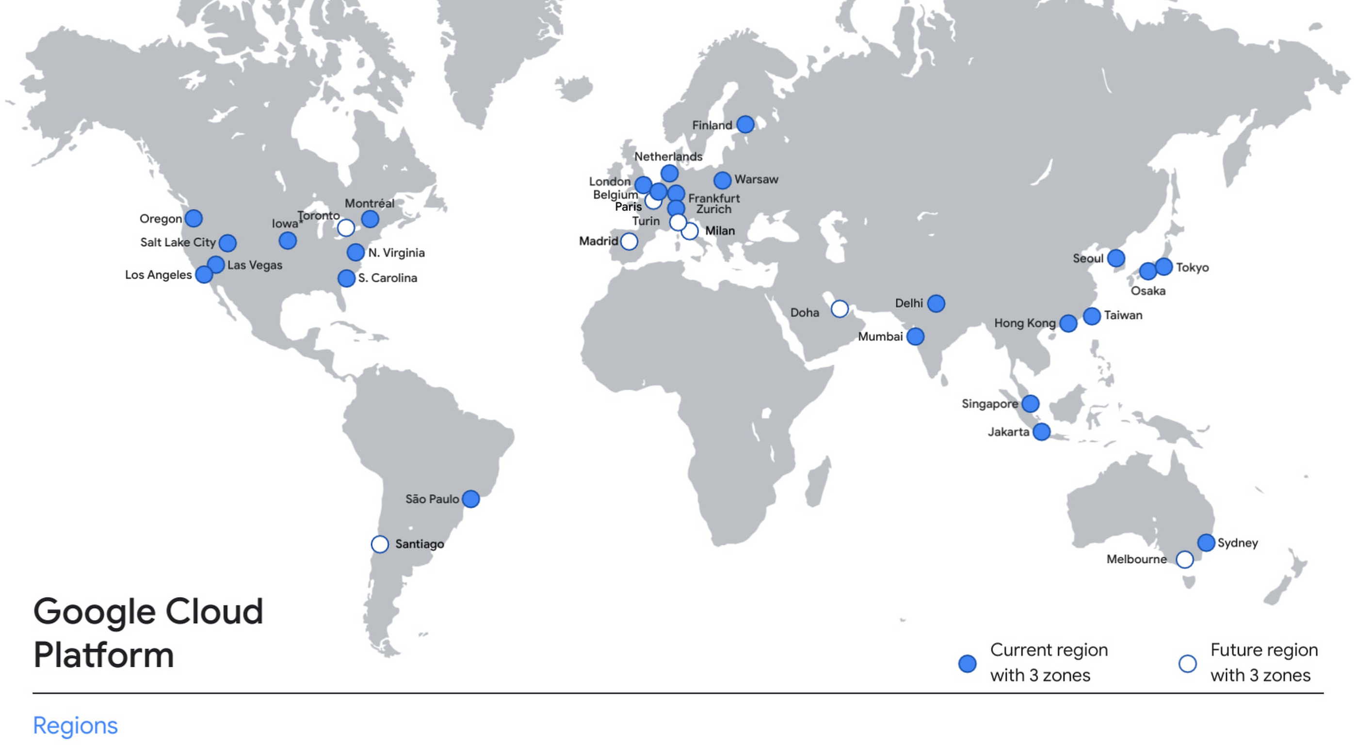
With this new region, Google Cloud customers operating in India also benefit from low latency and high performance of their cloud-based workloads and data. Designed for high availability, the region opens with three availability zones to protect against service disruptions, and offers a portfolio of key products, including Compute Engine, App Engine, Google Kubernetes Engine, Cloud Bigtable, Cloud Spanner, and BigQuery.
Supporting India’s recovery with training and education
Google and Google Cloud will also continue to support our customers with people and education programs. We’re investing in local talent and the local developer community to help enterprises digitally transform and support economic recovery.
Through the India Digitization Fund, we expanded our efforts to support India’s recovery from COVID-19—in particular, through programs to support education and small businesses. In addition to expanding internet access, and investments to help start-ups accelerate India’s digital transformation, we’ve grown our Grow with Google efforts. Businesses can access digital tools to maintain business continuity, find resources like quick help videos, and learn digital skills—in both English and in Hindi.
Helping customers build their transformation clouds
Google Cloud is here to support businesses, helping them get smarter with data, deploy faster, connect more easily with people and customers throughout the globe, and protect everything that matters to their businesses. The cloud region in Delhi NCR offers new technology and tools that can be a catalyst for this change. To learn more, visit the Google Cloud locations page, and be sure to watch the region launch event here.
8428
Of your peers have already watched this video.
21:00 Minutes
The most insightful time you'll spend today!
Journey to Transformation and Modernization with Google’s Distributed Cloud
Google Cloud has been leading the way of helping businesses make most from their cloud investments to drive digital transformation through modern application platforms that cater to today’s customer needs. Watch the video from the Next ’21 to explore three areas where companies are supported by Google Cloud throughout their cloud evolution journey–cloud migration and modernization, extension of services and engineering practices to hybrid and multicloud environments, and delivery of high performance with planet scale distributed infrastructure. Also, learn how Google Cloud is equipped for more complex and unique use cases, from datacenter to the edge. Hear the strategies and customer stories that can help your business modernize people, processes, and applications to fully leverage Google’s distributed cloud!
Recommendations for Modelling SAP Data inside BigQuery
8440
Of your peers have already read this article.
4:00 Minutes
The most insightful time you'll spend today!
Over the past few years, many organizations have experienced the benefits of migrating their SAP solutions to Google Cloud. But this migration can do more than reduce IT maintenance costs and make data more secure. By leveraging BigQuery, SAP customers can complement their SAP investments and gain fresh insights by consolidating enterprise data and easily extending it with powerful datasets and machine learning from Google.
BigQuery is a leading cloud data warehouse, fully managed and serverless, and allows for massive scale, supporting petabyte-scale queries at super-fast speeds. It can easily combine SAP data with additional data sources, such as Google Analytics or Salesforce, and its built-in machine learning lets users operationalize machine learning models using standard SQL — all at a comparatively low cost.
If your SAP-powered organization is looking to supercharge its analytics with the strength of BigQuery, read on for considerations and recommendations for modeling with SAP data. These guidelines are based on our real-world implementation experience with customers and can serve as a roadmap to the analytics capabilities your business needs.
Considerations for data replication
Like most technology journeys, this one should start with a business objective. Keeping your intended business value and goals in mind is critical to making the right decisions in the early steps of the design process.
When it comes to replicating the data from an SAP system into BigQuery, there are multiple ways to do it successfully. Decide which method will work best for your organization by answering these questions:
- Does your business need real-time data? Will you need to time travel into past data?
- Which external datasets will you need to join with the replicated data?
- Are the source structures or business logic likely to change? Will you be migrating the SAP source systems any time soon? For instance, will you be moving from SAP ECC to SAP S/4HANA?
You’ll also need to determine whether replication should be done on a table-by-table basis or whether your team can source from pre-built logic. This decision, along with other considerations such as licensing, will influence which replication tool you should use.
Replicating on a table-by-table basis
Replicating tables, especially standard tables in their raw form, allows sources to be reused and ensures more stability of the source structure and functional output. For example, the SAP table for sales order headers (VBAK) is very unlikely to change its structure across different versions of SAP, and the logic that writes to it is also unlikely to change in a way that affects a replicated table.
Something else to consider: Reconciliation between the source system and the landing table in BigQuery is linear when comparing raw tables, which helps avoid issues in consolidation exercises during critical business processes, such as period-end closing. Since replicated tables aren’t aggregated or subject to process-specific data transformation, the same replicated columns can be reused in different BigQuery views. You can, for instance, replicate the MARA table (the material master) once and use it in as many models as needed.
Replicating pre-built logic
If you replicate pre-built models, such as those from SAP extractors or CDS views, you don’t need to build the logic in BigQuery, since you’re using existing logic. Some of these extraction objects have embedded delta mechanisms, which may complement a replication tool that can’t handle deltas. This will save initial development time, but it can also lead to challenges if you create new columns, or if customizations or upgrades change the logic behind the extraction.
It’s also important to note that different extraction processes may transform and load the same source columns multiple times, which creates redundancy in BigQuery and can lead to higher maintenance needs and costs. However, replicating pre-built models may still be a good choice, since doing so can be especially useful for logic that tends to be immutable, such as flattening a hierarchy, or logic that is highly complex.
How you approach replication will also depend on your long-term plans and other key factors — for example, the availability (and curiosity) of your developers, and the time or effort they can put into applying their SQL knowledge to a new data warehouse.
With either replication approach, bear in mind when designing your replication process that BigQuery is meant to be an append-always database — so post-processing of data and changes will be required in both cases.
Processing data changes
The replication tool you choose will also determine how data changes are captured (known as CDC – change data capture). If the replication tool allows for it (for example as SAP SLT does) the same patterns described in the CDC with BigQuery documentation also apply to SAP data.
Because some data, like transactions, are known to be less static than others (e.g., master data), you need to decide what should be scanned in real time, what will require immediate consistency, and what can be processed in batches to manage costs. This decision will be based on the reporting needs from the business.
Consider the SAP table BUT000, containing our example master data for business partners, where we have replicated changes from an SAP ERP system:
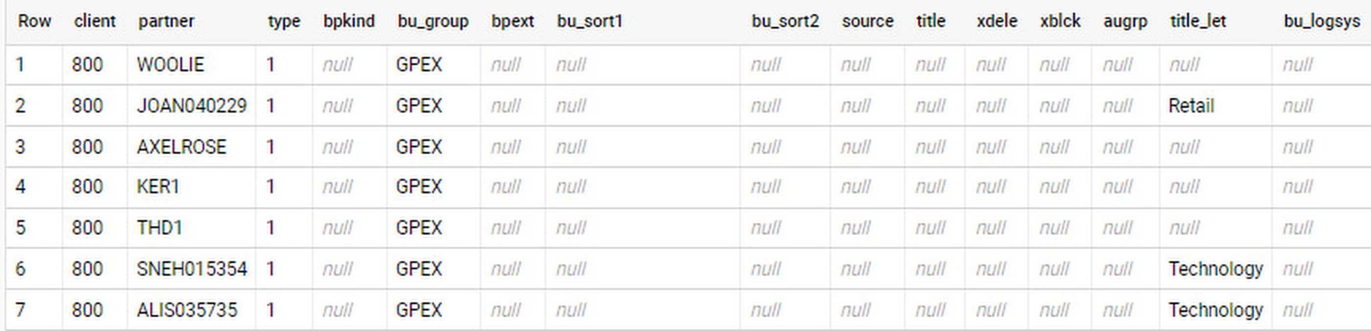
In an append-always replication in BigQuery, all updates are received as new records. For example, deleting a record in the source will be represented as a new record in BigQuery with a deletion flag. This applies to whether the records are coming from raw tables like BUT000 itself or pre-aggregated data, as from a BW extractor or a CDS view.
Let’s take a closer look at data coming particularly from the partners “LUCIA” and “RIZ”. The operation flag tells us whether the new record in BigQuery is an insert (I), update (U) or deletion (D), while the timestamps help us identify the latest version of our business partner.
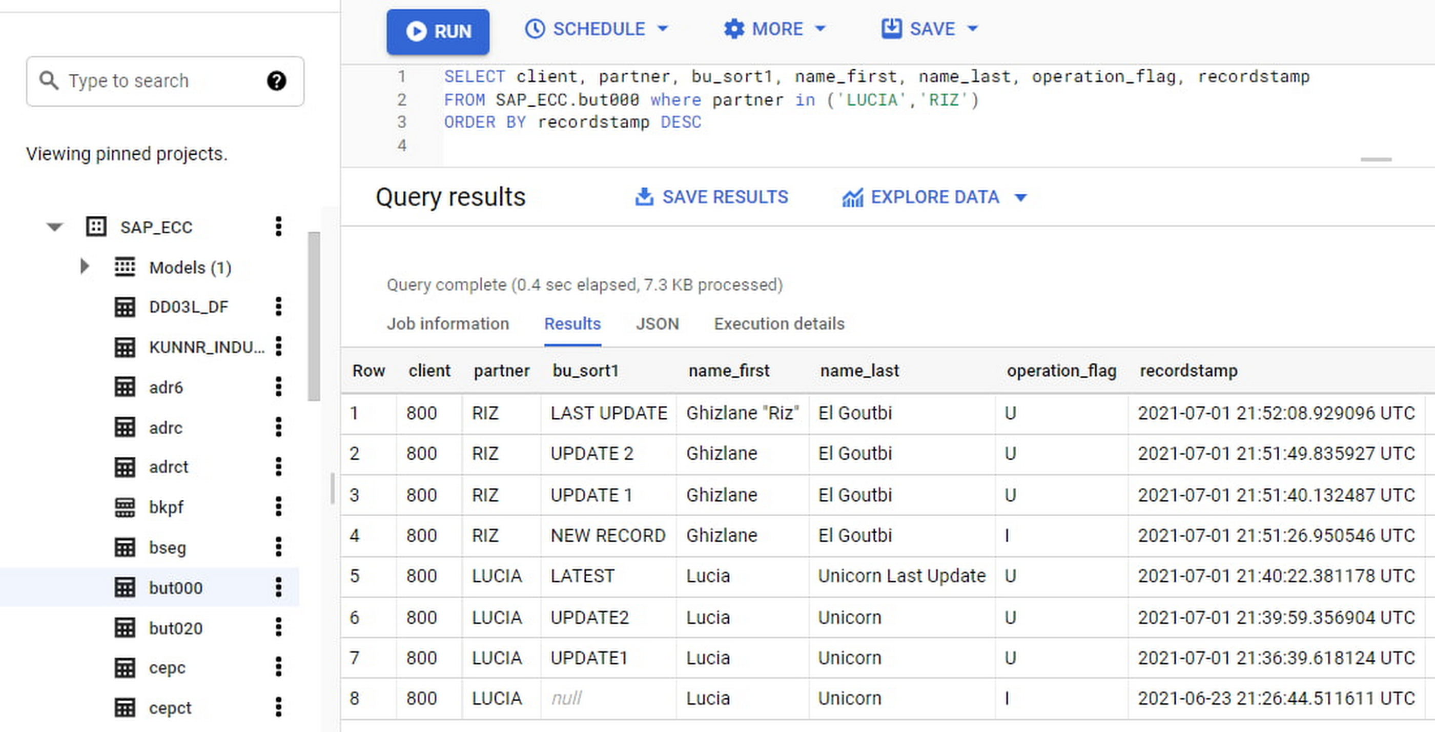
If we want to find the latest updated record for the partners LUCIA and RIZ, this is what the query would look like:
SELECT partner,ARRAY_AGG(i1 ORDER BY i1.recordstamp DESC LIMIT 1) AS rowFROM SAP_ECC.but000 i1WHERE partner in ('LUCIA','RIZ')GROUP BY partner
With the following result:
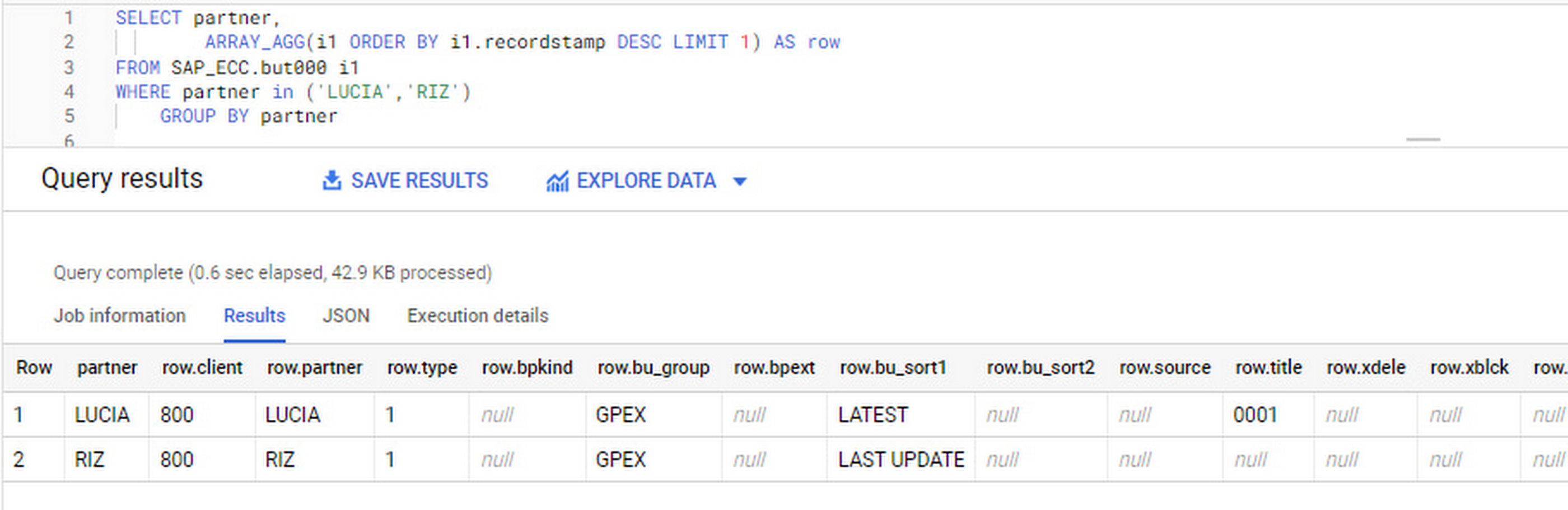
After identifying stale records for “LUCIA” and “RIZ” business partners, we can proceed to deleting all stale records for “LUCIA” if we do not want to retain the history. In this example, we are using a different table to which the same replication has been done, for the purpose of comparison and to check that all stale records have been deleted for the selection made and that we only kept last updated records. For example:
DELETE SAP_HANA.but000 i1WHEREi1.recordstamp < TIMESTAMP_SUB(CURRENT_TIMESTAMP(), INTERVAL 3 HOUR) ANDi1.recordstamp < (SELECT MAX(recordstamp) FROM SAP_HANA.but000 i2WHEREi1.partner = i2.partnerand partner="LUCIA")
You can also use the following query to retrieve stale records for “LUCIA” partner before moving forward with deletion
SELECT partner, operation_flag, recordstamp FROM SAP_HANA.but000 i1WHEREi1.recordstamp < TIMESTAMP_SUB(CURRENT_TIMESTAMP(), INTERVAL 3 HOUR)ANDi1.recordstamp < (SELECT MAX(recordstamp) FROM SAP_HANA.but000 i2WHEREi1.partner = i2.partnerand partner="LUCIA")
Which produces all of the records, except the latest update:

Partitioning and clustering
To limit the number of records scanned in a query, save on cost and achieve the best performance possible, you’ll need to take two important steps: determine partitions and create clusters.
Partitioning
A partitioned table is one that’s divided into segments, called partitions, which make it easier to manage and query your data. Dividing a large table into smaller partitions improves query performance and controls costs because it reduces the number of bytes read by a query.
You can partition BigQuery tables by:
- Time-unit column: Tables are partitioned based on a “timestamp,” “date,” or “datetime” column in the table.
- Ingestion time: Tables are partitioned based on the timestamp recorded when BigQuery ingested the data.
- Integer range: Tables are partitioned based on an integer column.
Partitions are enabled when the table is created, as in the example below. A great tip is to always include the partition filter as shown on the left-hand side of the query.

Clustering
Clustering can be created on top of partitioned tables by applying the fields that are likely to be used for filtering. When you create a clustered table in BigQuery, the table data is automatically organized based on the contents of one or more of the columns in the table’s schema. The columns you specify are then used to colocate related data.
Clustering can improve the performance of certain query types — for example, queries that use filter clauses or that aggregate data. It makes a lot of sense to use them for large tables such as ACDOCA, the table for accounting documents in SAP S/4HANA. In this case, the timestamp could be used for partitioning, and common filtering fields such as the ledger, company code, and fiscal year could be used to define the clusters.
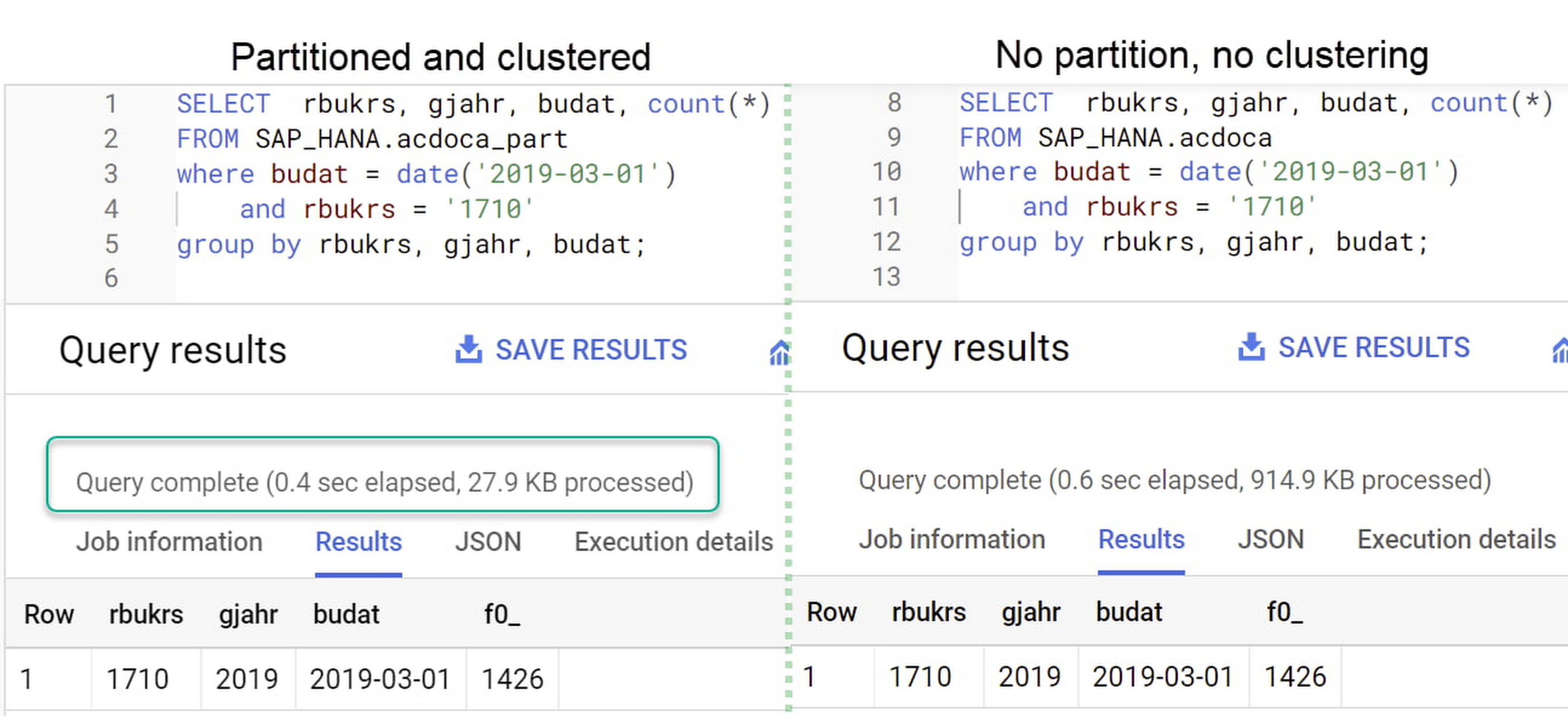
A great feature is that BigQuery will also periodically recluster the data automatically.
Materialized views
In BigQuery, materialized views are precomputed views that periodically cache the results of a query for better performance and efficiency. BigQuery uses precomputed results from materialized views and, whenever possible, reads only the delta changes from the base table to compute up-to-date results quickly. Materialized views can be queried directly or can be used by the BigQuery optimizer to process queries to the base table.
Queries that use materialized views are generally completed faster and consume fewer resources than queries that retrieve the same data only from the base table. If workload performance is an issue, materialized views can significantly improve the performance of workloads that have common and repeated queries. While materialized views currently only support single tables, they are very useful common and frequent aggregations like stock levels or order fulfillment.
Further tips on performance optimization while creating select statements can be found in the documentation for optimizing query computation.
Deployment pipeline and security
For most of the work you’ll do in BigQuery, you’ll normally have at least two delivery pipelines running — one for the actual objects in BigQuery and the other to keep the data staging, transforming, and updated as intended within the change-data-capture flows. Note that you can use most existing tools for your Continuous Integration / Continuous Deployment (CI/CD) pipeline — one of the benefits of using an open system like BigQuery. But, if your organization is new to CI/CD pipelines, this is a great opportunity to gradually gain experience. A good place to start is to read our guide for setting up a CI/CD pipeline for your data-processing workflow.
When it comes to access and security, most end-users will only have access to the final version of the BigQuery views. While row and column-level security can be applied, as in the SAP source system, separation of concerns can be taken to the next level by splitting your data across different Google Cloud projects and BigQuery datasets. While it’s easy to replicate data and structures across your datasets, it’s a good idea to define the requirements and naming conventions early in the design process so you set it up properly from the start.
Start driving faster and more insightful analytics
The best piece of advice we can give you is this: Try it yourself. Anyone with SQL knowledge can get started using the free BigQuery tier. New customers get $300 in free credits to spend on Google Cloud during the first 90 days. All customers get 10 GB storage and up to 1 TB queries/month, completely free of charge. In addition to discovering the massive processing capabilities, embedded machine learning, multiple integration tools, and cost benefits, you’ll soon discover how BigQuery can simplify your analytics tasks.
If you need additional assistance, our Google Cloud Professional Services Organization (PSO) and Customer Engineers will be happy to help show you the best path forward for your organization. For anything else, contact us at cloud.google.com/contact.
More Relevant Stories for Your Company
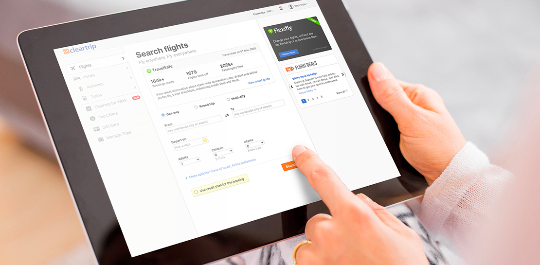
How Cleartrip.com is leveraging Google Cloud to survive the slump in the travel industry
With the novel coronavirus COVID-19 sweeping across continents and fatalities climbing every day, it was only a matter of time before countries closed their borders to contain its spread. In the wake of this decision, travel and tourism, the linchpins of many economies, were among the worst affected. According to

Cart.com to Transform e-Commerce for Brands Globally
The ecommerce playing field has been hard to navigate for most retailers, and Cart.com is on a mission to change that. Traditionally, retailers needing to run their online store, order fulfillment, customer service, marketing, and other essential activities have had to cobble together systems to get the capabilities they need

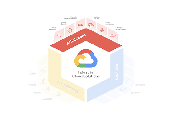
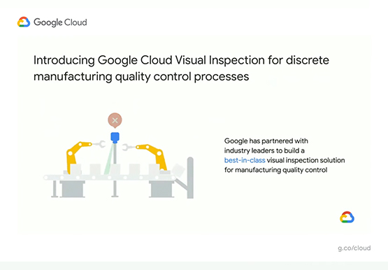

Driving Business Transformation in Manufacturing, Industrial, and Transportation Using Google Cloud and AI/ML
Google Cloud partners closely with manufacturing, industrial, and transportation organizations to drive business transformation. In this video, Mandeep Waraich, Head of Product - Industrial AI, Google Cloud, shares customer stories as well as Google Cloud’s differentiated AI products and solutions. Waraich covers the current state of automation and industrial efficiency
Unlocking Data Value: Latest Data Platforms and Announcements at the Next 21
Today at Google Cloud Next we are announcing innovations that will enable data teams to simplify how they work with data and derive value from it faster. These new solutions will help organizations build modern data architectures with real-time analytics to power innovative, mission-critical, data-driven applications. Too often, even the best minds
