How to Enhance Incremental Pipeline Performance while Ingesting Data into BigQuery

How-to

How to Enhance Incremental Pipeline Performance while Ingesting Data into BigQuery

6329

Of your peers have already read this article.

3:00 Minutes

The most insightful time you'll spend today!

When ingesting data into BigQuery, you can enhance data ingestion pipelines from large and frequently updated table in the source system. Refer the blog with examples and tips listed to streamline your journey with BigQuery.

When you build a data warehouse, the important question is how to ingest data from the source system to the data warehouse. If the table is small you can fully reload a table on a regular basis, however, if the table is large a common technique is to perform incremental table updates. This post demonstrates how you can enhance incremental pipeline performance when you ingest data into BigQuery.

Setting up a standard incremental data ingestion pipeline

We will use the below example to illustrate a common ingestion pipeline that incrementally updates a data warehouse table. Let’s say that you ingest data into BigQuery from a large and frequently updated table in the source system, and you have Staging and Reporting areas (datasets) in BigQuery.

The Reporting area in BigQuery stores the most recent, full data that has been ingested from the source system tables. Usually you create the base table as a full snapshot of the source system table. In our running example, we use BigQuery public data as the source system and create reporting.base_table as shown below. In our example each row is identified by a unique key which consists of two columns: block_hash and log_index.

  CREATE TABLE reporting.base_table  --156 GB processed
PARTITION BY TIMESTAMP_TRUNC(block_timestamp, DAY) AS
SELECT log_index, data, topics, block_timestamp, block_hash
FROM bigquery-public-data.crypto_ethereum.logs
WHERE block_timestamp BETWEEN TIMESTAMP '2020-01-01' AND TIMESTAMP '2020-11-30';

In data warehouses it is common to partition a large base table by a datetime column that has a business meaning. For example, it may be a transaction timestamp, or datetime when some business event happened, etc. The idea is that data analysts who use the data warehouse usually need to analyze only some range of dates and rarely need the full data. In our example, we partition the base table by block_timestamp which comes from the source system.

After ingesting the initial snapshot you need to capture changes that happen in the source system table and update the reporting base table accordingly. This is when the Staging area comes into the picture. The staging table will contain captured data changes that you will merge into the base table. Let’s say that in our source system on a regular basis we have a set of new rows and also some updated records. In our example we mock the staging data as follows: first, we create new data, than we mock the updated records:

  CREATE TABLE staging.load_delta AS --5 GB processed
SELECT log_index, data, topics, block_timestamp, block_hash
FROM bigquery-public-data.crypto_ethereum.logs
WHERE block_timestamp BETWEEN TIMESTAMP '2020-12-01' AND TIMESTAMP '2020-12-07';
 
INSERT INTO staging.load_delta --2 GB processed
SELECT log_index, CONCAT(data, RAND()), topics, block_timestamp, block_hash
FROM bigquery-public-data.crypto_ethereum.logs TABLESAMPLE SYSTEM (5 PERCENT)
WHERE block_timestamp BETWEEN TIMESTAMP '2020-10-01' AND TIMESTAMP '2020-11-30';

Next, the pipeline merges the staging data into the base table. It joins two tables by unique key and than updates the changed value or inserts a new row

  MERGE INTO reporting.base_table T --161 GB processed
USING staging.load_delta S
ON T.block_hash = S.block_hash
 AND T.log_index = S.log_index
WHEN MATCHED THEN UPDATE SET 
  T.data = S.data
WHEN NOT MATCHED THEN INSERT (log_index, data, topics, block_timestamp, block_hash)
VALUES (log_index, data, topics, block_timestamp, block_hash);

It is often the case that the staging table contains keys from various partitions but the number of those partitions are relatively small. It holds, for instance, because in the source system the recently added data may get changed due to some initial errors or ongoing processes but older records are rarely updated. However, when the above MERGE gets executed, BigQuery scans all partitions in the base table and processes 161 GB of data. You might add additional join condition on block_timestamp:

  MERGE INTO reporting.base_table T --161 GB processed
USING staging.load_delta S
ON T.block_hash = S.block_hash
 AND T.log_index = S.log_index
 AND T.block_timestamp = S.block_timestamp
WHEN MATCHED THEN UPDATE SET 
  T.data = S.data
WHEN NOT MATCHED THEN INSERT (log_index, data, topics, block_timestamp, block_hash)
VALUES (log_index, data, topics, block_timestamp, block_hash);

But BigQuery would still scan all partitions in the base table because condition T.block_timestamp = S.block_timestamp is a dynamic predicate and BigQuery doesn’t automatically push such predicates down from one table to another in MERGE.

Can you improve the MERGE efficiency by making it scan less data? The answer is Yes.

As described in the MERGE documentation, pruning conditions may be located in a subquery filter, a merge_condition filter, or a search_condition filter. In this post we show how you can leverage the first two. The main idea is to turn a dynamic predicate into a static predicate.

Steps to enhance your ingestion pipeline

The initial step is to compute the range of partitions that will be updated during the MERGE and store it in a variable. As was mentioned above, in data ingestion pipelines, staging tables are usually small so the cost of the computation is relatively low.

  DECLARE src_range STRUCT<date_min TIMESTAMP, date_max TIMESTAMP> --115 MB processed
DEFAULT(SELECT STRUCT(
  MIN(block_timestamp) AS date_min,  
  MAX(block_timestamp) AS date_max) FROM staging.load_delta);

Based on your existing ETL/ELT pipeline, you can add the above code as-is to your pipeline or you can compute date_min, data_max as part of some already existing transformation step. Alternatively, date_min, data_max can be computed on the Source System side while capturing the next ingestion data batch.

After computing date_min, date_max you pass those values to the MERGE statement as static predicates. There are several ways to enhance the MERGE and prune partitions in the base table based on precomputed date_min, data_max.

If your initial MERGE statement uses a subquery, you can incorporate a new filter into it:

  BEGIN 
DECLARE src_range STRUCT<date_min TIMESTAMP, date_max TIMESTAMP> --115 MB processed
DEFAULT(SELECT STRUCT(
  MIN(block_timestamp) AS date_min,  
  MAX(block_timestamp) AS date_max) FROM staging.load_delta);

MERGE INTO reporting.base_table T --41 GB processed
USING (
  SELECT *
  FROM staging.load_delta
  WHERE block_timestamp BETWEEN src_range.date_min AND src_range.date_max) S 
ON T.block_hash = S.block_hash
 AND T.log_index = S.log_index
 AND T.block_timestamp = S.block_timestamp
WHEN MATCHED THEN UPDATE SET 
  T.data = S.data
WHEN NOT MATCHED THEN INSERT (log_index, data, topics, block_timestamp, block_hash)
VALUES (log_index, data, topics, block_timestamp, block_hash);
END;

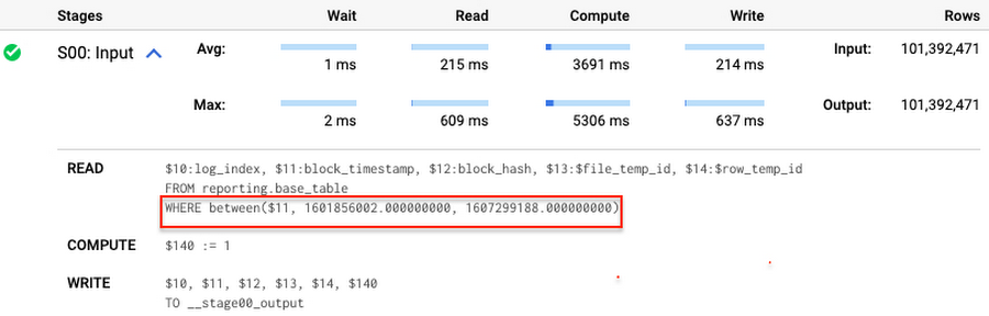
Note that you add the static filter to the staging table and keep T.block_timestamp = S.block_timestamp to convey to BigQuery that it can push that filter to the base table. This MERGE processes 41 GB of data in contrast to the initial 161 GB. You can see in the query plan that BigQuery pushes the partition filter from the staging table to the base table:

This type of optimization, when a pruning condition is pushed from a subquery to a large partitioned or clustered table, is not unique for MERGE. It also works for other types of queries. For instance:

  SELECT * -- 41 GB processed
FROM reporting.base_table T
INNER JOIN staging.load_delta S
ON T.block_hash = S.block_hash
 AND T.log_index = S.log_index
 AND T.block_timestamp = S.block_timestamp
WHERE S.block_timestamp BETWEEN TIMESTAMP '2020-10-05' AND TIMESTAMP '2020-12-07'

And you can check the query plan to verify that BigQuery pushed down the partition filter from one table to another.

Moreover, for SELECT statements, BigQuery can automatically infer a filter predicate on a join column and push it down from one table to another if your query meets the following criteria:

The target table must be clustered or partitioned.
The result size of the other table, i.e. after applying all filters, must qualify for broadcast join. Namly, the result set must be relatively small, less than ~100MB.

In our running example, reporting.base_table is partitioned by block_timestamp. If you define a selective filter on staging.load_delta and join two tables, you can see an inferred filter on the join key pushed to the target table

  SELECT * 
FROM reporting.base_table T
INNER JOIN staging.load_delta S
ON T.block_timestamp = S.block_timestamp
WHERE S.block_hash = '0x0c1caa16b34d94843aabfebc0d5a961db358135988f7498a6fdc450ad55f0870'

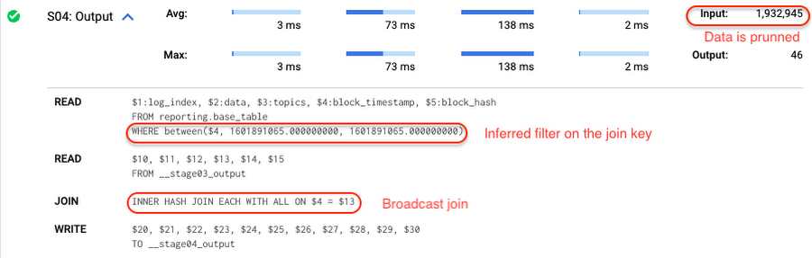
There is no requirement to join tables by partitioning or clustering key to kick off this type of optimization. However, in this case the pruning effect on the target table would be less significant.

But let us get back to the pipeline optimizations. Another way to enhance MERGE is to modify the merge_condition filter by adding static predicate on the base table:

  BEGIN 
DECLARE src_range STRUCT<date_min TIMESTAMP, date_max TIMESTAMP> --115 MB processed
DEFAULT(SELECT STRUCT(
  MIN(block_timestamp) AS date_min,  
  MAX(block_timestamp) AS date_max) FROM staging.load_delta);

MERGE INTO reporting.base_table T --41 GB processed
USING staging.load_delta S
ON T.block_hash = S.block_hash
 AND T.log_index = S.log_index
 AND T.block_timestamp BETWEEN src_range.date_min AND src_range.date_max
WHEN MATCHED THEN UPDATE SET 
  T.data = S.data
WHEN NOT MATCHED THEN INSERT (log_index, data, topics, block_timestamp, block_hash)
VALUES (log_index, data, topics, block_timestamp, block_hash);
END;

To summarize, here are the steps that you can perform to enhance incremental ingestion pipelines in BigQuery. First you compute the range of updated partitions based on the small staging table. Next, you tweak the MERGE statement a bit to let BigQuery know to prune data in the base table.

All the enhanced MERGE statements scanned 41 GB of data, and setting up the src_range variable took 115 MB. Compare it with the initial 161 GB scan. Moreover, given that computing src_range may be incorporated into some existing transformation in your ETL/ELT, it results in a good performance improvement which you can leverage in your pipelines.

In this post we described how to enhance data ingestion pipelines by turning dynamic filter predicates into static predicates and letting BiQuery prune data for us. You can find more tips on BigQuery DML tuning here.

Special thanks to Daniel De Leo, who helped with examples and provided valuable feedback on this content.

Case Study

Google Cloud Helps Northwell Health to Boost Caregiver Productivity and Access to Right Care Using AI

7969

Of your peers have already read this article.

2:00 Minutes

The most insightful time you'll spend today!

Northwell Health leverages Google Cloud products to build AI models that help identify patients with high probability of developing lung cancer, and guide the oncologists with those insights to deliver appropriate follow-up care. Read more!

Lung cancer is the leading cause of cancer death in the United States and like any cancer, early detection is crucial to survival. Screening at-risk populations is an important part of reducing mortality, and if concerning nodules are found on imaging, further testing may be required. Today, we’ll share how Northwell Health uses Google Cloud products such as Cloud Healthcare APIs and BigQuery to increase caregiver productivity and deliver better care for patients with findings that indicate potential development of lung cancer.

Northwell is New York’s largest healthcare provider

Northwell Health is New York’s largest healthcare provider with 23 hospitals and nearly 800 outpatient facilities. Northwell’s nearly 4,000 doctors care for millions of patients each year, and at this scale, there is an immense amount of healthcare data to manage. To better manage and leverage this data, Northwell Health partnered with Google Cloud starting in 2018.

Enabling caregivers to spend more time with patients

Nic Lorenzen, the lead developer of Northwell Emerging Technology and Innovation team, has a mission to put together data for caregivers in a way that makes sense. It is no secret that inefficient electronic health records systems have a negative impact on a physician’s ability to deliver quality care. Traditional EHRs have information distributed across many tabs, which forces caregivers to spend considerable time at the computer trying to find information. Moreover, speed of care matters. If care is delayed, patients may have to spend more time in the hospital and may suffer worse health outcomes.

To solve this problem, Nic’s team focused on giving caregivers the most relevant pieces of data at the right time by developing an intelligent clinician rounding app. The data needed to derive these insights can depend on the caregiver’s role–a nurse cares about different things than a cardiologist. This system aggregates multiple data sources, and provides patient-specific insights to caregivers.

This system would not have been possible before with traditional EHRs and data warehouses that have proprietary data models and rarely sync data in real time. Now with data easily accessible through Google Cloud’s Healthcare solutions, Nic’s team can deliver the right clinical information to the right people instantly. These days, Nic says, “instead of spending 75% of our time dealing with architecting the underlying platforms, we spend 75% of our time focused on higher value use cases for clinicians and patients. Google Cloud’s Healthcare solutions have greatly improved our developer productivity and time to value.”

Caregivers have found this new system to be a game changer.Before the implementation of this system, caregivers would spend, on average, seven to nine minutes finding the data needed to make medical decisions for one patient. Now, that aggregated information is delivered to a caregiver’s mobile device in less than a second.

Ensuring patients get the right care with the power of AI

There are a number of reasons why patients might not get the care that they need. For example, patients today can go to multiple hospitals and clinics settings, and coordinating care across multiple facilities is complex. Regional hospitals and clinics have their own siloed view of their data, so pertinent information gathered by one clinic might not be seen by another. These gaps in clinical data lead to gaps in patient care.

When a patient gets radiologic imaging, they may have findings unrelated to the reason they initially got the imaging. For example, a chest CT for a car accident might reveal an incidental lung nodule that could be cancerous. Unfortunately, research shows that a large portion of patients do not get follow up for these incidental findings because it isn’t the primary reason why the patient is seeing a doctor. Moreover, social determinants of health are a factor that affects which patients receive follow-up care. Identifying these patients and providing the necessary follow up care prevents adverse events related to delayed detection of cancer.

*Source: https://commons.wikimedia.org/wiki/File:LungMets2008.jpg*

With Cloud Healthcare solutions, Northwell built an AI model to identify these patients so that oncologists can appropriately follow up with patients who have findings suspicious for lung cancer. The AI model detects incidental pulmonary nodules in radiology reports so that doctors can then contact the patients that need follow-up care. Nic says his team was able to build this system in a week: “Google Cloud did a lot of heavy-lifting for us and allowed us to get to the AI applications much faster. It allowed us to build a platform that just works.”

Healthcare systems can now rapidly generate healthcare insights with one end-to-end solution, Google Cloud Healthcare Data Engine. It builds on and extends the core capabilities of the Google Cloud Healthcare API to make healthcare data more immediately useful by enabling an interoperable, longitudinal record of patient data. Northwell Health uses Google Cloud as the core of their platform, enabling their developers to create solutions to the most pressing healthcare problems.

Special thanks to Kalyan Pamarthy, Product Management Lead on Cloud Healthcare and Natural Language APIs for contributing to this blog post.

Blog

Dataflow is getting better with Dataflow Prime, Dataflow Go, and Dataflow ML

3191

Of your peers have already read this article.

2:30 Minutes

The most insightful time you'll spend today!

Introducing three big releases that make the Dataflow faster, easier and accessible. With this major development, Team Google will be able to achieve its goal to democratize the power of big data, real time streaming, and ML/AI for all developers.

By the end of 2024, 75% of enterprises will shift from piloting to operationalizing artificial intelligence according to IDC, yet the growing complexity of data types, heterogeneous data stacks and programming languages make this a challenge for all data engineers. With the current economic climate, doing more with cheaper costs and higher efficiency have also become a key consideration for many organizations.

Today, we are pleased to announce three major releases that bring the power of Google Cloud’s Dataflow to more developers for expanded use cases and higher data processing workloads, while keeping the costs low, as part of our goal to democratize the power of big data, real time streaming, and ML/AI for all developers, everywhere.

The three big Dataflow releases we’re thrilled to announce in general availability are:

Dataflow Prime – Dataflow Prime takes the serverless, no-operation benefits of Dataflow to a totally new level. Dataflow Prime allows users to take advantage of both horizontal autoscaling (more machines) and vertical autoscaling (larger machines with more memory) automatically for your streaming data processing workloads, with batch coming in the near future. With Dataflow Prime, pipelines are more efficient, enabling you to apply the insights in real time.

Dataflow Go – Dataflow Go provides native support for Go, a rapidly growing programming language thanks to its flexibility, ease of use and differentiated concepts, for both batch and streaming data processing workloads. With Apache Beam’s unique multi-language model, Dataflow Go pipelines can leverage the well adopted, best-in-class performance provided by the wide range of Java I/O connectors with ML transforms and I/O connectors from Python coming soon.

Dataflow ML – Speaking of ML transforms, Dataflow now has added out of the box support for running PyTorch and scikit-learn models directly within the pipeline. The new RunInference transform enables simplicity by allowing models to be used in production pipelines with very little code. These features are in addition to Dataflow’s existing ML capabilities such as GPU support and the pre and post processing system for ML training, either directly or via frameworks such as Tensorflow Extended (TFX).

We’re so excited to make Dataflow even better. With the world’s only truly unified batch and streaming data processing model provided by Apache Beam, the wide support for ML frameworks, and the unique cross-language capabilities of the Beam model, Dataflow is becoming ever easier, faster, and more accessible for all data processing needs.

Getting started

To get started with Dataflow Go easily, see the Quickstart and download the Go SDK.
To learn more about Dataflow Prime, see the documentation.
To learn more about Dataflow ML and RunInference, read about the new RunInference Beam transform on the Apache Beam website.

Interested in running a proof of concept using your own data? Talk to your Google Cloud sales contact for hands-on workshop opportunities or sign up here.

10164

Of your peers have already watched this video.

1:00 Minutes

The most insightful time you'll spend today!

How-to

Predict User Churn on Gaming Apps with Google Analytics Data using BigQuery ML

User retention can be a major challenge for mobile game developers. According to the Mobile Gaming Industry Analysis in 2019, most mobile games only see a 25% retention rate for users after the first day. To retain a larger percentage of users after their first use of an app, developers can take steps to motivate and incentivize certain users to return. But to do so, developers need to identify the propensity of any specific user returning after the first 24 hours.

In this blog post, we will discuss how you can use BigQuery ML to run propensity models on Google Analytics 4 data from your gaming app to determine the likelihood of specific users returning to your app.

You can also use the same end-to-end solution approach in other types of apps using Google Analytics for Firebase as well as apps and websites using Google Analytics 4. To try out the steps in this blogpost or to implement the solution for your own data, you can use this Jupyter Notebook.

Using this blog post and the accompanying Jupyter Notebook, you’ll learn how to:

Explore the BigQuery export dataset for Google Analytics 4
Prepare the training data using demographic and behavioural attributes
Train propensity models using BigQuery ML
Evaluate BigQuery ML models
Make predictions using the BigQuery ML models
Implement model insights in practical implementations

Google Analytics 4 (GA4) properties unify app and website measurement on a single platform and are now default in Google Analytics. Any business that wants to measure their website, app, or both, can use GA4 for a more complete view of how customers engage with their business. With the launch of Google Analytics 4, BigQuery export of Google Analytics data is now available to all users. If you are already using a Google Analytics 4 property, you can follow this guide to set up exporting your GA data to BigQuery.

Once you have set up the BigQuery export, you can explore the data in BigQuery. Google Analytics 4 uses an event-based measurement model. Each row in the data is an event with additional parameters and properties. The Schema for BigQuery Export can help you to understand the structure of the data.

In this blogpost, we use the public sample export data from an actual mobile game app called “Flood It!” (Android, iOS) to build a churn prediction model. But you can use data from your own app or website.

Here’s what the data looks like. Each row in the dataset is a unique event, which can contain nested fields for event parameters.

  SELECT *
FROM `firebase-public-project.analytics_153293282.events_*`
TABLESAMPLE SYSTEM (1 PERCENT)

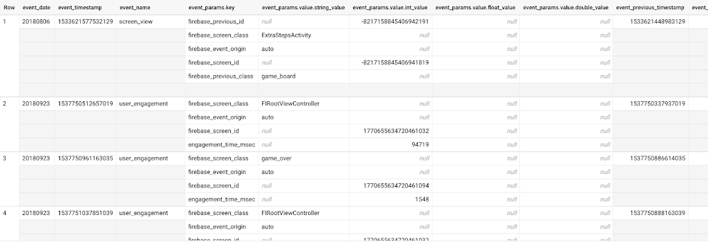
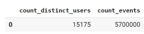
This dataset contains 5.7M events from over 15k users.

  SELECT 
    COUNT(DISTINCT user_pseudo_id) as count_distinct_users,
    COUNT(event_timestamp) as count_events
FROM
  `firebase-public-project.analytics_153293282.events_*

Our goal is to use BigQuery ML on the sample app dataset to predict propensity to user churn or not churn based on users’ demographics and activities within the first 24 hours of app installation.

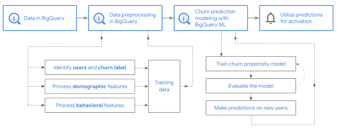
In the following sections, we’ll cover how to:

Pre-process the raw event data from GA4
1. Identify users & the label feature
2. Process demographic features
3. Process behavioral features
Train classification model using BigQuery ML
Evaluate the model using BigQueryML
Make predictions using BigQuery ML
Utilize predictions for activation

Pre-process the raw event data

You cannot simply use raw event data to train a machine learning model as it would not be in the right shape and format to use as training data. So in this section, we’ll go through how to pre-process the raw data into an appropriate format to use as training data for classification models.

This is what the training data should look like for our use case at the end of this section:

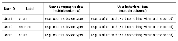
Notice that in this training data, each row represents a unique user with a distinct user ID (user_pseudo_id).

Identify users & the label feature

We first filtered the dataset to remove users who were unlikely to return the app anyway. We defined these ‘bounced’ users as ones who spent less than 10 mins with the app. Then we labeled all remaining users:

churned: No event data for the user after 24 hours of first engaging with the app.
returned: The user has at least one event record after 24 hours of first engaging with the app.

For your use case, you can have a different definition of bounce and churning. Also you can even try to predict something else other than churning, e.g.:

whether a user is likely to spend money on in-game currency
likelihood of completing n-number of game levels
likelihood of spending n amount of time in-game etc.

In such cases, label each record accordingly so that whatever you are trying to predict can be identified from the label column.

From our dataset, we found that ~41% users (5,557) bounced. However, from the remaining users (8,031), ~23% (1,883) churned after 24 hours:

  SELECT
    bounced,
    churned, 
    COUNT(churned) as count_users
FROM
    bqmlga4.returningusers
GROUP BY 1,2
ORDER BY bounced

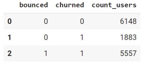
To create these bounced and churned columns, we used the following snippet of SQL code.

  ...
#churned = 1 if last_touch within 24 hr of app installation, else 0
IF (user_last_engagement < TIMESTAMP_ADD(user_first_engagement, 
      INTERVAL 24 HOUR),
    1,
    0 ) AS churned,
#bounced = 1 if last_touch within 10 min, else 0
IF (user_last_engagement <= TIMESTAMP_ADD(user_first_engagement, 
      INTERVAL 10 MINUTE),
    1,
    0 ) AS bounced,
...

You can view the Jupyter Notebook for the full query used for materializing the bounced and churned labels.

Process demographic features

Next, we added features both for demographic data and for behavioral data spanning across multiple columns. Having a combination of both demographic data and behavioral data helps to create a more predictive model.

We used the following fields for each user as demographic features:

geo.country
device.operating_system
device.language

A user might have multiple unique values in these fields — for example if a user uses the app from two different devices. To simplify, we used the values from the very first user engagement event.

  CREATE OR REPLACE VIEW bqmlga4.user_demographics AS (
  WITH first_values AS (
      SELECT
          user_pseudo_id,
          geo.country as country,
          device.operating_system as operating_system,
          device.language as language,
          ROW_NUMBER() OVER (PARTITION BY user_pseudo_id ORDER BY event_timestamp DESC) AS row_num
      FROM `firebase-public-project.analytics_153293282.events_*`
      WHERE event_name="user_engagement"
      )
  SELECT * EXCEPT (row_num)
  FROM first_values
  WHERE row_num = 1 #first engagement
);

Process behavioral features

There is additional demographic information present in the GA4 export dataset, e.g. app_info, device, event_params, geo etc. You may also send demographic information to Google Analytics through each hit via user_properties. Furthermore, if you have first-party data on your own system, you can join that with the GA4 export data based on user_ids.

To extract user behavior from the data, we looked into the user’s activities within the first 24 hours of first user engagement. In addition to the events automatically collected by Google Analytics, there are also the recommended events for games that can be explored to analyze user behavior. For our use case, to predict user churn, we counted the number of times the follow events were collected for a user within 24 hours of first user engagement:

user_engagement
level_start_quickplay
level_end_quickplay
level_complete_quickplay
level_reset_quickplay
post_score
spend_virtual_currency
ad_reward
challenge_a_friend
completed_5_levels
use_extra_steps

The following query shows how these features were calculated:

  WITH
  events_first24hr AS (
    SELECT
      e.*
    FROM
      `firebase-public-project.analytics_153293282.events_*` e
    JOIN
      bqmlga4.returningusers r
      ON
        e.user_pseudo_id = r.user_pseudo_id
    WHERE
      TIMESTAMP_MICROS(e.event_timestamp) <= r.ts_24hr_after_first_engagement
  )
SELECT
  user_pseudo_id,
  SUM(IF(event_name = 'user_engagement', 1, 0)) AS cnt_user_engagement,
  # ... repeated for all behavior data ... 
  SUM(IF(event_name = 'use_extra_steps', 1, 0)) AS cnt_use_extra_steps,
FROM
  events_first24hr
GROUP BY
  1

View the notebook for the query used to aggregate and extract the behavioral data. You can use different sets of events for your use case. To view the complete list of events, use the following query:

  SELECT
    event_name,
    COUNT(event_name) as event_count
FROM
    `firebase-public-project.analytics_153293282.events_*`
GROUP BY 1
ORDER BY
   event_count DESC

After this we combined the features to ensure our training dataset reflects the intended structure. We had the following columns in our table:

User ID:
- user_pseudo_id
Label:
- churned
Demographic features
- country
- device_os
- device_language
Behavioral features
- cnt_user_engagement
- cnt_level_start_quickplay
- cnt_level_end_quickplay
- cnt_level_complete_quickplay
- cnt_level_reset_quickplay
- cnt_post_score
- cnt_spend_virtual_currency
- cnt_ad_reward
- cnt_challenge_a_friend
- cnt_completed_5_levels
- cnt_use_extra_steps
- user_first_engagement

At this point, the dataset was ready to train the classification machine learning model in BigQuery ML. Once trained, the model will output a propensity score between churn (churned=1) or return (churned=0) indicating the probability of a user churning based on the training data.

Train classification model

When using the CREATE MODEL statement, BigQuery ML automatically splits the data between training and test. Thus the model can be evaluated immediately after training (see the documentation for more information).

For the ML model, we can choose among the following classification algorithms where each type has its own pros and cons:

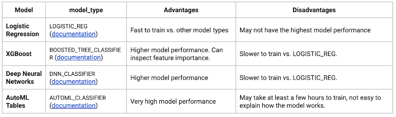
Often logistic regression is used as a starting point because it is the fastest to train. The query below shows how we trained the logistic regression classification models in BigQuery ML.

  CREATE OR REPLACE MODEL bqmlga4.churn_logreg
TRANSFORM(
  EXTRACT(MONTH from user_first_engagement) as month,
  EXTRACT(DAYOFYEAR from user_first_engagement) as julianday,
  EXTRACT(DAYOFWEEK from user_first_engagement) as dayofweek,
  EXTRACT(HOUR from user_first_engagement) as hour,
  * EXCEPT(user_first_engagement, user_pseudo_id)
)
OPTIONS(
  MODEL_TYPE="LOGISTIC_REG",
  INPUT_LABEL_COLS=["churned"]
) AS
SELECT
  *
FROM
  bqmlga4.train

We extracted month, julianday, and dayofweek from datetimes/timestamps as one simple example of additional feature preprocessing before training. Using TRANSFORM() in your CREATE MODEL query allows the model to remember the extracted values. Thus, when making predictions using the model later on, these values won’t have to be extracted again. View the notebook for the example queries to train other types of models (XGBoost, deep neural network, AutoML Tables).

Evaluate model

Once the model finished training, we ran ML.EVALUATE to generate precision, recall, accuracy and f1_score for the model:

  SELECT
  *
FROM
  ML.EVALUATE(MODEL bqmlga4.churn_logreg)

The optional THRESHOLD parameter can be used to modify the default classification threshold of 0.5. For more information on these metrics, you can read through the definitions on precision and recall, accuracy, f1-score, log_loss and roc_auc. Comparing the resulting evaluation metrics can help to decide among multiple models.Furthermore, we used a confusion matrix to inspect how well the model predicted the labels, compared to the actual labels. The confusion matrix is created using the default threshold of 0.5, which you may want to adjust to optimize for recall, precision, or a balance (more information here).

  SELECT
  expected_label,
  _0 AS predicted_0,
  _1 AS predicted_1
FROM
  ML.CONFUSION_MATRIX(MODEL bqmlga4.churn_logreg)

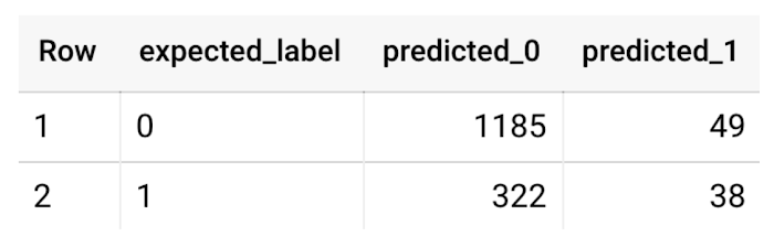
This table can be interpreted in the following way:

Make predictions using BigQuery ML

Once the ideal model was available, we ran ML.PREDICT to make predictions. For propensity modeling, the most important output is the probability of a behavior occurring. The following query returns the probability that the user will return after 24 hrs. The higher the probability and closer it is to 1, the more likely the user is predicted to return, and the closer it is to 0, the more likely the user is predicted to churn.

  SELECT
  user_pseudo_id,
  returned,
  predicted_returned,
  predicted_returned_probs[OFFSET(0)].prob as probability_returned
FROM
  ML.PREDICT(MODEL bqmlga4.churn_logreg,
  (SELECT * FROM bqmlga4.train)) #can be replaced with a proper test dataset

Utilize predictions for activation

Once the model predictions are available for your users, you can activate this insight in different ways. In our analysis, we used user_pseudo_id as the user identifier. However, ideally, your app should send back the user_id from your app to Google Analytics. In addition to using first-party data for model predictions, this will also let you join back the predictions from the model into your own data.

You can import the model predictions back into Google Analytics as a user attribute. This can be done using the Data Import feature for Google Analytics 4. Based on the prediction values you can Create and edit audiences and also do Audience targeting. For example, an audience can be users with prediction probability between 0.4 and 0.7, to represent users who are predicted to be “on the fence” between churning and returning.
For Firebase Apps, you can use the Import segments feature. You can tailor user experience by targeting your identified users through Firebase services such as Remote Config, Cloud Messaging, and In-App Messaging. This will involve importing the segment data from BigQuery into Firebase. After that you can send notifications to the users, configure the app for them, or follow the user journeys across devices.
Run targeted marketing campaigns via CRMs like Salesforce, e.g. send out reminder emails.

You can find all of the code used in this blogpost in the Github repository:

https://github.com/GoogleCloudPlatform/analytics-componentized-patterns/tree/master/gaming/propensity-model/bqml

What’s next?

Continuous model evaluation and re-training

As you collect more data from your users, you may want to regularly evaluate your model on fresh data and re-train the model if you notice that the model quality is decaying.

Continuous evaluation—the process of ensuring a production machine learning model is still performing well on new data—is an essential part in any ML workflow. Performing continuous evaluation can help you catch model drift, a phenomenon that occurs when the data used to train your model no longer reflects the current environment.

To learn more about how to do continuous model evaluation and re-train models, you can read the blogpost: Continuous model evaluation with BigQuery ML, Stored Procedures, and Cloud Scheduler

More resources

If you’d like to learn more about any of the topics covered in this post, check out these resources:

Or learn more about how you can use BigQuery ML to easily build other machine learning solutions:

Let us know what you thought of this post, and if you have topics you’d like to see covered in the future! You can find us on Twitter at @polonglin and @_mkazi_.Thanks to reviewers: Abhishek Kashyap, Breen Baker, David Sabater Dinter.

Blog

Ahead of the Curve: 5 Data and AI Trends Set to Shape 2023

2260

Of your peers have already read this article.

4:00 Minutes

The most insightful time you'll spend today!

Google Cloud's 2023 Data and AI Trends report lists five trends: unified data cloud, open data ecosystems, embracing AI tipping point, insights infusion, and exploring unknown data. Learn how to integrate these trends into your business strategy.

How will your organization manage this year’s data growth and business requirements? Your actions and strategies involving data and AI will improve or undermine your organization’s competitiveness in the months and years to come. Our teams at Google Cloud have an eye on the future as we evolve our strategies to protect technology choice, simplify data integration, increase AI adoption, deliver needed information on demand, and meet security requirements.

Google Cloud worked with* IDC on multiple studies involving global organizations across industries in order to explore how data leaders are successfully addressing key data and AI challenges. We compiled the results in our 2023 Data and AI Trends report. In it, you’ll find the metrics-rich research behind the top five data and AI trends, along with tips and customer examples for incorporating them into your plans.

1: Show data silos the door

Given the increasing volumes of data we’re all managing, it’s no surprise that siloed transactional databases and warehousing strategies can’t meet modern demands. Organizations want to improve how they store, manage, analyze, and govern all their data, while reducing costs. They also want to eliminate conflicting insights from replicated data and empower everyone with fresh data.

A unified data cloud enables the integration of data and insights into transformative digital experiences and better decision making.

Andi Gutmans, GM and VP of Engineering for Databases, Google Cloud

Tweet this quote

In the report, you can learn how to adopt a unified data cloud that supports every stage of the data lifecycle so that you can improve data usage, accessibility, and governance. Inform your strategy by drawing on organizations’ examples such as a data fabric that improves customer experiences by connecting more than 80 data silos, as well as other unified data clouds that save money and simplify growth.

2: Usher in the age of the open data ecosystem

Data is the key to unlocking AI, speeding up development cycles, and increasing ROI. To protect against data and technology lock-in, more organizations are adopting open source software and open APIs.

Organizations want the freedom to create a data cloud that includes all formats of data from any source or cloud.

-Gerrit Kazmaier, VP and GM, Data & Analytics, Google Cloud

Tweet this quote

Understand how you can simplify data integration, facilitate multicloud analytics, and use the technologies you want with an open data ecosystem, as described in the report. Learn from metrics about global open source adoption and public dataset usage. And explore how global companies adopted open data ecosystems to improve patient outcomes, increase website traffic by 25%, and cut operating costs by 90%.

3: Embrace the AI tipping point

Pulling useful information out of data is easier with AI and ML. Not only can you identify patterns and answer questions faster but the technologies also make it easier to solve problems at scale.

We’ve reached the AI tipping point. Whether people realize it or not, we’re already using applications powered by AI—every day. Social media platforms, voice assistants, and driving services are easy examples.

June Yang, VP, Cloud AI and Industry Solutions, Google Cloud

Tweet this quote

Organizations share how they’re reaching their goals using AI and ML by empowering “citizen data scientists” and having them focus on small wins first. Gain tips from Yang and other experts for developing your AI strategy. And read how organizations achieve outcomes such as a reduction of 7,400 tons per year in carbon emissions and a more than 200% increase in ROI from ad spend by using pattern recognition and other AI capabilities.

4: Infuse insights everywhere

Yesterday’s BI solutions have led to outdated insights and user fatigue with the status quo, based on generic metrics and old information. Research shows that as new tools come online, expectations for BI are changing, with companies revising their strategies to improve decision making, speed up the development of new revenue streams, and increase customer acquisition and retention by providing individuals with needed information on demand.

Organizations are equipping business decision-makers with the tools they need to incorporate required insights into their everyday workflows.

Kate Wright, Senior Director, Product Management, Google Cloud

Tweet this quote

In the report, you’ll discover why and how data leaders are rethinking their BI analytics strategies and applications to improve users’ trust and use of data in automated workflows, customizable dashboards, and on-demand reports. Global companies also share how they improve decision making with self-service BI, customer experiences with IoT analysis, and threat mitigation with embedded analytics.

5: Get to know your unknown data

Increasing data volumes can make it harder to know where and what data they store, which may create risk. Case in point: If a customer unexpectedly shares personally identifiable information during a recorded customer support call or chat session, that data might require specialized governance, which the standardized storage process may not provide.

If you don’t know what data you have, you cannot know that it’s accurately secured. You also don’t know what security risks you are incurring, or what security measures you need to take.

Anton Chuvakin, Senior Staff Security Consultant, Google Cloud

Tweet this quote

Check out the report to learn about data security risks that are often overlooked and how to develop proactive governance strategies for your sensitive data. You can also read how global organizations have increased customer trust and productivity by improving how they discover, classify, and manage their structured and unstructured data.

Be ready for what’s next

What’s exciting about these trends is that they’re enabling organizations across industries to realize very different goals using their choice of technologies. And although all the trends depend on each other, research shows you can realize measurable benefits whether you adopt one or all five.

Review the report yourself and learn how you can refine your organization’s data and AI strategies by drawing on the collective insights, experiences, and successes of more than 800 global organizations.

Case Study

Real-time analytics for on-time delivery: Mercado Libre

3048

Of your peers have already read this article.

1:30 Minutes

The most insightful time you'll spend today!

The onset of the pandemic drove exponential order growth for Mercado Libre. Read to know how Google BigQuery and Looker combined provide near real-time data monitoring, analytics for transportation networks and deliver valuable insights.

Iteration and innovation fuel the data-driven culture at Mercado Libre. In our first post, we presented our continuous intelligence approach, which leverages BigQuery and Looker to create a data ecosystem on which people can build their own models and processes.

Using this framework, the Shipping Operations team was able to build a new solution that provided near real-time data monitoring and analytics for our transportation network and enabled data analysts to create, embed, and deliver valuable insights.

The challenge

Shipping operations are critical to success in e-commerce, and Mercado Libre’s process is very complex since our organization spans multiple countries, time zones, and warehouses, and includes both internal and external carriers. In addition, the onset of the pandemic drove exponential order growth, which increased pressure on our shipping team to deliver more while still meeting the 48-hour delivery timelines that customers have come to expect.

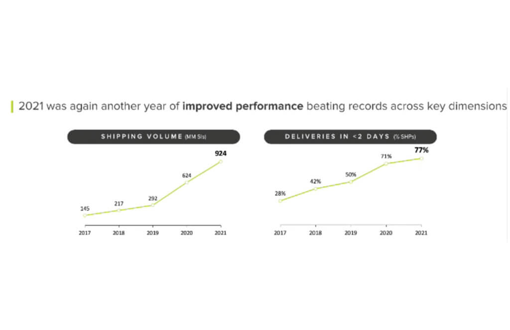
This increased demand led to the expansion of fulfillment centers and cross-docking centers, doubling and tripling the nodes of our network (a.k.a. meli-net) in the leading countries where we operate. We also now have the largest electric vehicle fleet in Latin America and operate domestic flights in Brazil and Mexico.

We previously worked with data coming in from multiple sources, and we used APIs to bring it into different platforms based on the use case. For real-time data consumption and monitoring, we had Kibana, while historical data for business analysis was piped into Teradata. Consequently, the real-time Kibana data and the historical data in Teradata were growing in parallel, without working together. On one hand, we had the operations team using real-time streams of data for monitoring, while on the other, business analysts were building visualizations based on the historical data in our data warehouse.

This approach resulted in a number of problems:

The operations team lacked visibility and required support to build their visualizations. Specialized BI teams became bottlenecks.
Maintenance was needed, which led to system downtime.
Parallel solutions were ungoverned (the ops team used an Elastic database to store and work with attributes and metrics) with unfriendly backups and data bounded for a period of time.
We couldn’t relate data entities as we do with SQL.

Striking a balance: real-time vs. historical data

We needed to be able to seamlessly navigate between real-time and historical data. To address this need, we decided to migrate the data to BigQuery, knowing we would leverage many use cases at once with Google Cloud.

Once we had our real-time and historical data consolidated within BigQuery, we had the power to make choices about which datasets needed to be made available in near real-time and which didn’t. We evaluated the use of analytics with different time windows tables from the data streams instead of the real-time logs visualization approach. This enabled us to serve near real-time and historical data utilizing the same origin.

We then modeled the data using LookML, Looker’s reusable modeling language based on SQL, and consumed the data through Looker dashboards and Explores. Because Looker queries the database directly, our reporting mirrored the near real-time data stored in BigQuery. Finally, in order to balance near real-time availability with overall consumption costs, we analyzed key use cases on a case-by-case basis to optimize our resource usage.

This solution prevented us from having to maintain two different tools and featured a more scalable architecture. Thanks to the services of GCP and the use of BigQuery, we were able to design a robust data architecture that ensures the availability of data in near real-time.

Streaming data with our own Data Producer Model: from APIs to BigQuery

To make new data streams available, we designed a process which we call the “Data Producer Model” (“Modelo Productor de Datos” or MPD) where functional business teams can serve as data creators in charge of generating data streams and publishing them as related information assets we call “data domains”. Using this process, the new data comes in via JSON format, which is streamed into BigQuery. We then use a 3-tiered transformation process to convert that JSON into a partitioned, columnar structure.

To make these new data sets available in Looker for exploration, we developed a Java utility app to accelerate the development of LookML and make it even more fun for developers to create pipelines.

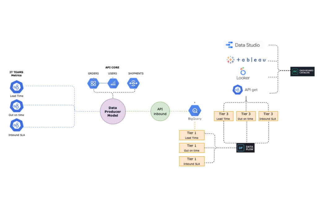
*The end-to-end architecture of our Data Producer Model.*

The complete “MPD” solution results in different entities being created in BigQuery with minimal manual intervention. Using this process, we have been able to automate the following:

The creation of partitioned, columnar tables in BigQuery from JSON samples
The creation of authorized views in a different GCP BigQuery project (for governance purposes)
LookML code generation for Looker views
Job orchestration in a chosen time window

By using this code-based incremental approach with LookML, we were able to incorporate techniques that are traditionally used in DevOps for software development, such as using Lams to validate LookML syntax as a part of the CI process and testing all our definitions and data with Spectacles before they hit production. Applying these principles to our data and business intelligence pipelines has strengthened our continuous intelligence ecosystem. Enabling exploration of that data through Looker and empowering users to easily build their own visualizations has helped us to better engage with stakeholders across the business.

The new data architecture and processes that we have implemented have enabled us to keep up with the growing and ever-changing data from our continuously expanding shipping operations. We have been able to empower a variety of teams to seamlessly develop solutions and manage third party technologies, ensuring that we always know what’s happening – and more critically – enabling us to react in a timely manner when needed.

Outcomes from improving shipping operations:

Today, data is being used to support decision-making in key processes, including:

Carrier Capacity Optimization
Outbound Monitoring
Air Capacity Monitoring

This data-driven approach helps us to better serve you -and everyone- who expects to receive their packages on-time according to our delivery promise. We can proudly say that we have improved both our coverage and speed, delivering 79% of our shipments in less than 48 hours in the first quarter of 2022.

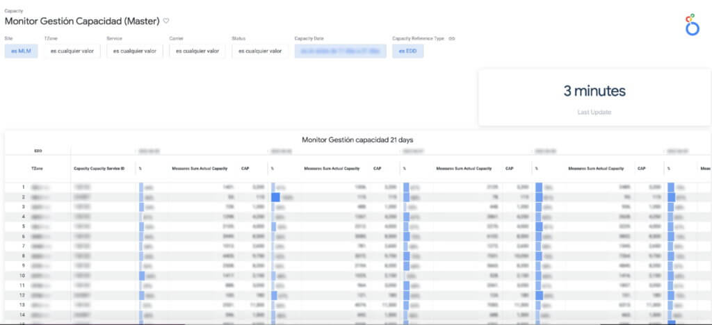
Here is a sneak peek into the data assets that we use to support our day-to-day decision making:

a. Carrier Capacity: Allows us to monitor the percentage of network capacity utilized across every delivery zone and identify where delivery targets are at risk in almost real time.

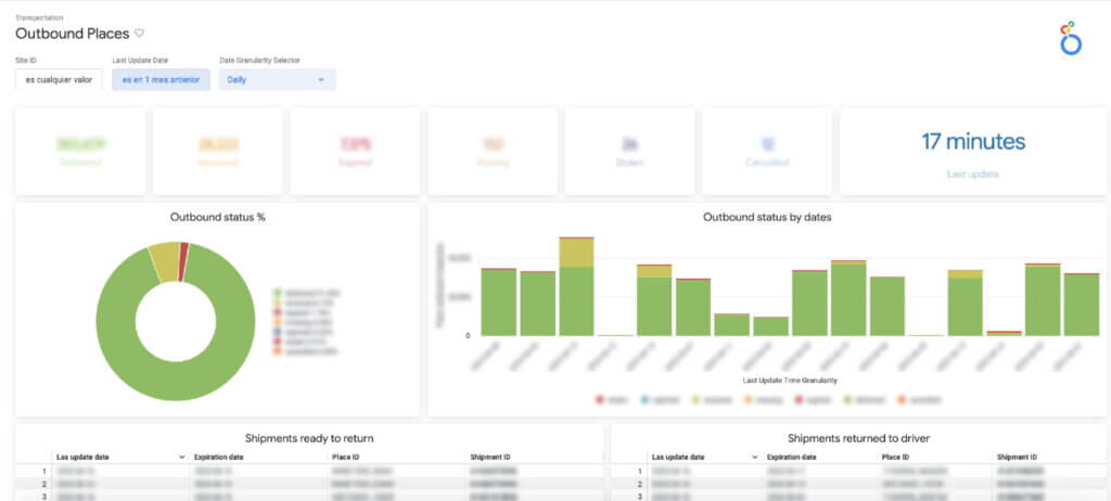
b. Outbound Places Monitoring: Consolidates the number of shipments that are destined for a place (the physical points where a seller picks up a package), enabling us to both identify places with lower delivery efficiency and drill into the status of individual shipments.

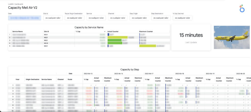
c. The Air Capacity Monitoring: Provides capacity usage monitoring for our aircrafts running each of our shipping routes.

Costs into the equation

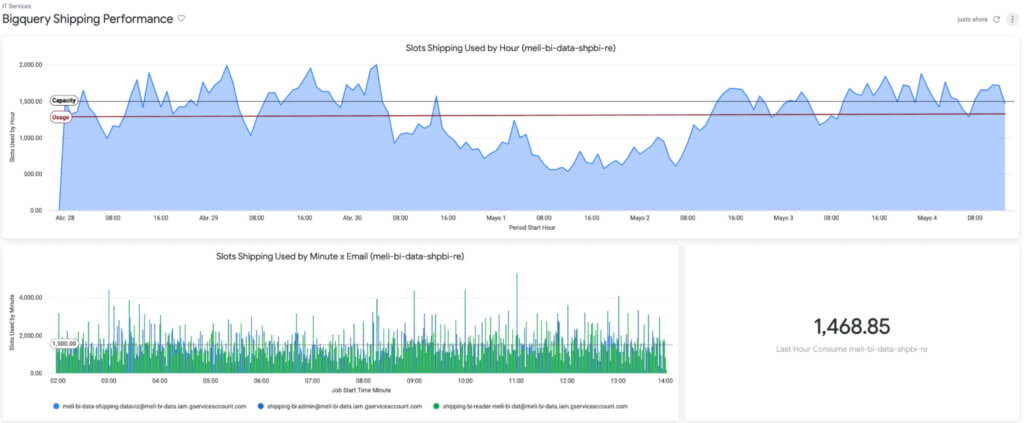
The combination of BigQuery and Looker also showed us something we hadn’t seen before: overall cost and performance of the system. Traditionally, developers maintained focus on metrics like reliability and uptime without factoring in associated costs.

By using BigQuery’s information schema, Looker Blocks, and the export of BigQuery logs, we have been able to closely track data consumption, quickly detect underperforming SQL and errors, and make adjustments to optimize our usage and spend.

Based on that, we know the Looker Shipping Ops dashboards generate a concurrency of more than 150 queries, which we have been able to optimize by taking advantage of BigQuery and Looker caching policies.

The challenges ahead

Using BigQuery and Looker has enabled us to solve numerous data availability and data governance challenges: single point access to near real-time data and to historical information, self-service analytics & exploration for operations and stakeholders across different countries & time zones, horizontal scalability (with no maintenance), and guaranteed reliability and uptime (while accounting for costs), among other benefits.

However, in addition to having the right technology stack and processes in place, we also need to enable every user to make decisions using this governed, trusted data. To continue achieving our business goals, we need to democratize access not just to the data but also to the definitions that give the data meaning. This means incorporating our data definitions with our internal data catalog and serving our LookML definitions to other data visualizations tools like Data Studio, Tableau or even Google Sheets and Slides so that users can work with this data through whatever tools they feel most comfortable using.

If you would like a more indepth look at how we made new data streams available from a process we designed called the “Data Producer Model” (“Modelo Productor de Datos” or MPD) register to attend our webcast on August 31.

While learning and adopting new technologies can be a challenge, we are excited to tackle this next phase, and we expect our users will be too, thanks to a curious and entrepreneurial culture. Are our teams ready to face new changes? Are they able to roll out new processes and designs? We’ll go deep on this in our next post.

Migrating From Oracle OLTP System to Cloud Spanner

Spanner uses certain concepts differently from other enterprise database management tools, so you might need to adjust your application to take full advantage of its capabilities. You might also need to supplement Spanner with other services from Google Cloud to meet your needs. Migration constraints When you migrate your application

“We are extremely pleased with Google Cloud Platform and Firebase. We have been able to differentiate ourselves from our competitors and provide an attractive option for users at a time when content and entertainment options are exploding. —Shibin Li, Co-Founder, Castbox

Research Reports

How Data Efficiency with Google Cloud Empower Governments to Make Data-first Decisions

Presently, every government agency has to take a hard look at their data capabilities and decide whether their current infrastructure supports their workflow. For many, it doesn't. Most data systems are developed with a strict set of parameters in mind before implementation, which can limit flexibility and long-term use. Particularly

33% Of global infrastructure business decision makers already support a dBaas deployment in production, and this will likely double over the next three to four years.

How-to

No More ‘Tab Game’ with Easy Tutorials on Google Cloud Console

When it comes to learning how to implement some technology, we all have our own version of what I call the "tab game"—that is, your setup for all the tabs and windows you need open at once. You may have several monitors so you can see documentation, your IDE, and

Blog

Unlocking the Potential of Advanced Analytics with BigQuery and Connected Vehicle Data

As software-defined vehicles continue to advance and the quantity of digital services grows to meet consumer demand, the data required to provide these services continue to grow as well. This makes automotive manufacturers and suppliers look for capabilities to log and analyze data, update applications, and extend commands to in-vehicle

SHOW MORE STORIES

	Sadhana Subramanian, Technology Decision Maker Technology Decision Maker Technology Decision Maker Technology Decision Maker Technology Decision Maker Technology Decision Maker Technology Decision Maker Technology Decision Maker
	Sadhana Subramanian, Technology Decision Maker
	Sadhana Subramanian, Technology Decision Maker
	Sadhana Subramanian, Technology Decision Maker
	Sadhana Subramanian, Technology Decision Maker
	Sadhana Subramanian, Technology Decision Maker
	Sadhana Subramanian, Technology Decision Maker
	Sadhana Subramanian, Technology Decision Maker

We’d like to know you better! Help us serve you stories that matter

Thank You!

Share with your teammates