





Guide for Measuring Cloud Spanner Performance for Your Custom Workload

4833
Of your peers have already read this article.
3:00 Minutes
The most insightful time you'll spend today!
Database migration to a new database platform or technology can be daunting for various reasons. One of the common concerns is database performance. It is hard to evaluate database performance early in the evaluation cycle without performing actual data migration and application changes. This becomes even more important in the case of Cloud Spanner where modernization is required at both the database and application layers.
The traditional approach to evaluate database performance is to deploy the application and database together, migrate historical data to the new database and then simulate load tests by running an application on the new database. Doing all this for an early performance evaluation of Cloud Spanner may feel like a lot of effort.
In this post, we will explore a middle ground to performance testing using JMeter. Performance test Cloud Spanner for a custom workload before making application code changes and executing data migration. More detailed step-by-step guide is published here.
Goals
- Estimate the number of Cloud Spanner nodes needed (and get a cost estimate).
- Performance test the most frequently used set of queries and transactions.
- Demonstrate the ability to scale horizontally.
- Better understand the optimizations needed for schema and sql queries.
- Determine latency of DML operations.
Limitations
- You cannot test using non-java client libraries.
- It is more complex to test non-jdbc compliant features like mutations, parallel reads etc.
Preparing for performance tests
- Identify top SQL queries, latency, frequency / hour and avg number of rows returned or updated for each. This information will also serve as a baseline for the current system.
- Determine Cloud Spanner region / multi-region deployment. Ideally, load should be generated from the Cloud Spanner instance’s leader region for minimum latency and best performance. Read Demystifying Cloud Spanner multi-region configurations for more details on various configurations of Cloud Spanner.
- Estimate the number of Cloud Spanner nodes required for a given workload based on (step 1). It is recommended to have a minimum of 2 nodes for linear scaling.
Note: Peak performance numbers of regional performance and multi regional performance are published. It is based on a 1KB single row transaction with no secondary indexes. - Request quota for Cloud Spanner nodes on a given region / multi-region. It can take up to 1 business day.
Setting up Cloud Spanner
Creating the schema for Cloud Spanner
You can use the following tools to generate a schema for Cloud Spanner if you are migrating from the following source databases. Alternatively, you can model the schema manually. Schema design has a huge performance impact, hence it is recommended to review the schema very carefully.
| Source | Target | Tool(s) | |
| 1. | MySQL / MariaDB | Cloud Spanner | HarbourBridgeStriim |
| 2. | Postgresql | Cloud Spanner | HarbourBridgeStriim |
| 3. | Oracle | Cloud Spanner | Striim |
| 4. | SQL Server | Cloud Spanner | Striim |
Note: Manual review and tuning of schema will be needed to optimize and mitigate potential hotspots. You will need to keep in mind schema design best practices when modeling your schema.
Populating seed data into Cloud Spanner
Performance of a database depends on the amount of data present. Existing data (and indexes) determines how much data is scanned on select queries and therefore performance. Hence, it is important to seed data into Cloud Spanner before performance testing.
For most realistic results, data should be migrated from an existing production source. Sometimes you cannot do that due to schema changes. One way is to utilize a custom ETL job to export and transform data and then import into Cloud Spanner. Another alternative could be to mock seed data using JMeter(More details in later sections).
JMeter performance tests
Writing Tests
JMeter will interact with Cloud Spanner just like your application. It will perform DML operations the same way as your application does. Hence, tests need to simulate production like transactions. For example if a transaction is made up of insert and/or update statements in several tables within transaction boundaries then JMeter should mimic the same.
JMeter has the following hierarchy:
Test Plan > Thread Group(s) > Sampler(s) (aka test)
Test plan is a top level component. It can contain global properties and libraries (like jdbc driver etc).
Thread Group(s) are representative of a database transaction. It contains one or more sampler(s). All the samplers within a thread group execute serially.
Sampler(s) should represent a single DML call. If your transaction needs to have multiple dml calls, you should create multiple samplers. Typically you will use JDBC Sampler for database calls. You can also use JSR 223 Sampler as described here, in case you need to use mutations or parallel reads etc. Results from one sampler can be passed to the next, as in real world application.
Executing tests and collecting results
JMeter tests should be executed as physically close to Cloud Spanner instances as possible to minimize network latency. Therefore it is best to execute them from Compute Engine (via private service connect) from the same region as the Cloud Spanner instance. In-case of multi region Cloud Spanner, GCE instances should be created in the Leader Region of the Cloud Spanner instance for lowest network latency.
JMeter should be executed via command line, it is a CPU intensive application so make sure you have allocated enough resources on the VM.
Refer to the Cloud Spanner monitoring dashboard to ensure that your Cloud Spanner instance’s CPU utilization is at or below the recommended values. In addition, use introspection tools to investigate performance issues with your database.
You might need to optimize your queries (add indexes) and re-execute tests in multiple waves to tune the performance as needed.
Try it yourself
Follow a detailed step by step tutorial on Measure Cloud Spanner performance test using JMeter to test Cloud Spanner performance yourself.
Quantum Metric Increases Business 10-fold

9263
Of your peers have already read this article.
5:30 Minutes
The most insightful time you'll spend today!
At Quantum Metric, we’re in the business of bringing our customers business insights that are based on customer experience data and analytics for mid-market and Fortune 500 companies.
Our software, powered by big data, machine intelligence, and Google Cloud, helps our customers identify, quantify, prioritize and measure opportunities to improve digital experiences.
As companies move to a more agile product lifecycle, including continuous deployment and continuous integration, they’re finding that it’s critical to receive perpetual quantified feedback and insights from their data in real time to understand where the largest opportunities exist.
Each year, billions of customer interactions are captured through browsers or mobile apps on PCs, tablets, and mobile devices. This data, fed into the Quantum Metric platform, can show if a customer had a password problem they couldn’t solve or struggled when trying to purchase something and abandoned their cart.
It also can show if the customer tried in vain to complete an online change to their service provider’s subscription, to reach tech support, or couldn’t find the size or color they were looking for while shopping online.
Most importantly, the Quantum Metric platform quantifies the business value of the issue, helping organizations prioritize where they can make the largest impact to their business.
Success overwhelms our initial architecture
Initially, the Quantum Metric experience analytics software ran on a MySQL open source relational database management system (RDBMS). The MySQL RDBMS worked great for simple queries, when there was a specific question to ask of the data.
Soon, though, we knew we needed to offer more advanced data science capabilities. Our bigger customers wanted to ask questions across very large data sets—days, weeks, months, and years worth of data. They wanted to pose iterative questions using complex filters to answer their most challenging business questions.
With more complex queries across more data, response times from our RDBMS went from 100 to 500 milliseconds to as long as 20 minutes.
That delay was slowing down our ability and time to insights, which also reduced the value we could provide to our customers, since iterative exploration and analysis requires real-time query responses. Because of the need for real-time responses, there were certain questions that we just weren’t able to ask of the data. It became clear that we needed a much more robust data warehouse solution.
There were also operational challenges with MySQL and massive-scale data ingestion. We spent a lot of time into the wee hours of the night and morning handling errors and recovering databases.
We tried to address these challenges by sharding, partitioning, and indexing the data to optimize for the types of questions customers were asking. But the problems were escalating and happening more often, from once a month across the customer base to monthly for at least 20 different customers.
We could tune the platform for today and tomorrow’s workload, with good guesses at where indexes could be used, but we simply couldn’t continue to horizontally scale MySQL in a cost-efficient and operationally efficient manner.
Speed breeds innovation
Once we started exploring options that could better scale with our business, we looked at NoSQL technologies like Cassandra (a partitioned row-store database), MySQL’s Column Store (a columnar store database), and Vertica (a columnar store database)—each with unique ways of handling data storage and accessibility.
But with high volumes of complex queries across large data stores, all of these solutions began to fail, bogged down with multiple, simultaneous users. We could have solved the problems with more raw compute and storage, but it would have been prohibitively expensive to run and require a large team to operate.
We then decided to try BigQuery, and it was transformative.
We connected our front end to BigQuery via APIs. Once data is 15 minutes old, it is automatically extracted, loaded, and transformed (ETL) to BigQuery.
We continuously update the legacy MySQL RDBMS so its data is integrated with BigQuery data when queries require real-time data. Most query response times are within 100-200 milliseconds, matching what we initially experienced with MySQL.
When traffic from our customers scales up, we can now scale on-demand to accommodate it, thanks to BigQuery’s hundreds of thousands of CPUs. Our customers no longer run into slow response times, and we’ve gained confidence that we can offer them—and their users—advanced insights and better experiences without delay.
More importantly, with this scale of query power, we were able to build data science algorithms into the platform, which iteratively query BigQuery based on the results, and help quantify the impact of a specific issue to a specific segment of users. Adding these capabilities was possible because of the massive scale of BigQuery.
In addition to new insights and fast response times, we wanted our customers to be able to ask complex questions using very simple language.
For example: “Show me high-loyalty customers, located in specific geographic areas, who visited the web site at least five times, based on specific campaigns, and never booked a seat on a flight.”
This was exactly the kind of query that was used by a major U.S. airline to understand the multi-million dollar impact of a failure affecting their most valuable customers: their high-loyalty members.
And this was all done while maintaining the highest standard of care of customer data and privacy by default, using multiple layers of encryption of data in transit, at rest, and a unique military-grade encryption approach. This approach encrypts PII, including even session cookies, with a RSA-2048 key available only to a select few and used for use cases such as fraud analysis.
It’s no exaggeration to say that BigQuery has totally transformed our business. It provides the petabyte scale and speed we were missing, in addition to taking care of operational maintenance, a task that was burying our team with MySQL.
We’re now able to support some of the largest companies in the world that require real-time, petabyte-scale analytics. That lets them serve more customers faster with higher quality, and take advantage of BigQuery’s power and scale to innovate.
There are other cloud solutions that can address petabyte analytics, but the most unique value proposition of BigQuery was its on-demand scaling and operational management, with extremely cost-effective pay-as-you-go billing. While today we are at a scale where we have round-the-clock querying needs, our early days had very sporadic query loads where we needed instant scale, then a long lull of nothing. The unique business model of BigQuery’s pay-by-bytes-scanned allowed us to have access to a massive-scale querying platform without breaking the bank.
Using BigQuery powers better customer experience and reduces purchasing friction
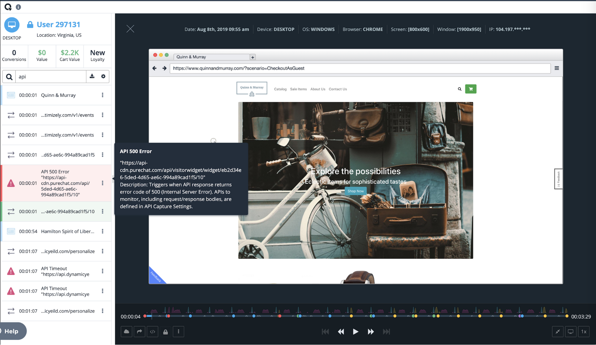
Among the many features of Quantum Metric is the ability to replay online customer sessions. In the example below from a mobile e-commerce site, each action is displayed chronologically. Why did this customer’s transaction fail?
Diving deeper, the session replay shows that the user tried to change the item quantity in the checkout cart, which resulted in a failed API call. Powered by BigQuery, Quantum Metric can then show how many other end users had this issue, with a simple click of “Show More Errors Like This.”
With BigQuery’s massive scale, Quantum Metric will then quantify the impact of that issue, so companies can prioritize which issues need attention immediately. If this is the issue that’s impacting the business the most, our customer can use a single click to open a Jira ticket, forwarding the discovery to their product and engineering teams. Those teams can then re-engineer the experience in near-real time, addressing the failed API call and cutting out the frustrating time it takes for engineers to reproduce the issue.
Once we had a powerful back end in BigQuery, we realized that Quantum Metric’s platform could be used to ask complex questions from vast datasets. We built some of the processes that data scientists use to formulate those queries right into our product.
For example, we added one series of processes to our platform to help customers understand whether a suspect issue is really impacting end-user experience. Is it something that should be prioritized and fixed? Does this really affect the user experience? Does it have financial impact? These and other questions can be pre-defined as a complex query in Quantum Metric to let our customer quickly gain insight on how an issue is impacting the business. Customers were blown away when they heard this was possible. It was the holy grail for what they were looking for in data science. It really sets us apart from our competition.
Today, with every company heavily dependent on data, those companies that can uncover and act on insights fastest are the ones that will succeed. BigQuery gives us the data warehouse platform we need to provide our customers with fast, reliable technology tools. It frees us from having to deal with the minutiae of technology infrastructure operations, so we can focus on finding and extracting the magic in customer data. With the power and scale of BigQuery, combined with the real-time capture of every user experience with 100% fidelity, we’re able to offer a self-service analytics platform that provides insights into digital journey friction points and acts as the indisputable arbitrator of truth.
How to Enhance Incremental Pipeline Performance while Ingesting Data into BigQuery

6327
Of your peers have already read this article.
3:00 Minutes
The most insightful time you'll spend today!
When you build a data warehouse, the important question is how to ingest data from the source system to the data warehouse. If the table is small you can fully reload a table on a regular basis, however, if the table is large a common technique is to perform incremental table updates. This post demonstrates how you can enhance incremental pipeline performance when you ingest data into BigQuery.
Setting up a standard incremental data ingestion pipeline
We will use the below example to illustrate a common ingestion pipeline that incrementally updates a data warehouse table. Let’s say that you ingest data into BigQuery from a large and frequently updated table in the source system, and you have Staging and Reporting areas (datasets) in BigQuery.

The Reporting area in BigQuery stores the most recent, full data that has been ingested from the source system tables. Usually you create the base table as a full snapshot of the source system table. In our running example, we use BigQuery public data as the source system and create reporting.base_table as shown below. In our example each row is identified by a unique key which consists of two columns: block_hash and log_index.
CREATE TABLE reporting.base_table --156 GB processedPARTITION BY TIMESTAMP_TRUNC(block_timestamp, DAY) ASSELECT log_index, data, topics, block_timestamp, block_hashFROM bigquery-public-data.crypto_ethereum.logsWHERE block_timestamp BETWEEN TIMESTAMP '2020-01-01' AND TIMESTAMP '2020-11-30';
In data warehouses it is common to partition a large base table by a datetime column that has a business meaning. For example, it may be a transaction timestamp, or datetime when some business event happened, etc. The idea is that data analysts who use the data warehouse usually need to analyze only some range of dates and rarely need the full data. In our example, we partition the base table by block_timestamp which comes from the source system.
After ingesting the initial snapshot you need to capture changes that happen in the source system table and update the reporting base table accordingly. This is when the Staging area comes into the picture. The staging table will contain captured data changes that you will merge into the base table. Let’s say that in our source system on a regular basis we have a set of new rows and also some updated records. In our example we mock the staging data as follows: first, we create new data, than we mock the updated records:
CREATE TABLE staging.load_delta AS --5 GB processedSELECT log_index, data, topics, block_timestamp, block_hashFROM bigquery-public-data.crypto_ethereum.logsWHERE block_timestamp BETWEEN TIMESTAMP '2020-12-01' AND TIMESTAMP '2020-12-07';INSERT INTO staging.load_delta --2 GB processedSELECT log_index, CONCAT(data, RAND()), topics, block_timestamp, block_hashFROM bigquery-public-data.crypto_ethereum.logs TABLESAMPLE SYSTEM (5 PERCENT)WHERE block_timestamp BETWEEN TIMESTAMP '2020-10-01' AND TIMESTAMP '2020-11-30';
Next, the pipeline merges the staging data into the base table. It joins two tables by unique key and than updates the changed value or inserts a new row
MERGE INTO reporting.base_table T --161 GB processedUSING staging.load_delta SON T.block_hash = S.block_hashAND T.log_index = S.log_indexWHEN MATCHED THEN UPDATE SETT.data = S.dataWHEN NOT MATCHED THEN INSERT (log_index, data, topics, block_timestamp, block_hash)VALUES (log_index, data, topics, block_timestamp, block_hash);
It is often the case that the staging table contains keys from various partitions but the number of those partitions are relatively small. It holds, for instance, because in the source system the recently added data may get changed due to some initial errors or ongoing processes but older records are rarely updated. However, when the above MERGE gets executed, BigQuery scans all partitions in the base table and processes 161 GB of data. You might add additional join condition on block_timestamp:
MERGE INTO reporting.base_table T --161 GB processedUSING staging.load_delta SON T.block_hash = S.block_hashAND T.log_index = S.log_indexAND T.block_timestamp = S.block_timestampWHEN MATCHED THEN UPDATE SETT.data = S.dataWHEN NOT MATCHED THEN INSERT (log_index, data, topics, block_timestamp, block_hash)VALUES (log_index, data, topics, block_timestamp, block_hash);
But BigQuery would still scan all partitions in the base table because condition T.block_timestamp = S.block_timestamp is a dynamic predicate and BigQuery doesn’t automatically push such predicates down from one table to another in MERGE.
Can you improve the MERGE efficiency by making it scan less data? The answer is Yes.
As described in the MERGE documentation, pruning conditions may be located in a subquery filter, a merge_condition filter, or a search_condition filter. In this post we show how you can leverage the first two. The main idea is to turn a dynamic predicate into a static predicate.
Steps to enhance your ingestion pipeline
The initial step is to compute the range of partitions that will be updated during the MERGE and store it in a variable. As was mentioned above, in data ingestion pipelines, staging tables are usually small so the cost of the computation is relatively low.
DECLARE src_range STRUCT<date_min TIMESTAMP, date_max TIMESTAMP> --115 MB processedDEFAULT(SELECT STRUCT(MIN(block_timestamp) AS date_min,MAX(block_timestamp) AS date_max) FROM staging.load_delta);
Based on your existing ETL/ELT pipeline, you can add the above code as-is to your pipeline or you can compute date_min, data_max as part of some already existing transformation step. Alternatively, date_min, data_max can be computed on the Source System side while capturing the next ingestion data batch.
After computing date_min, date_max you pass those values to the MERGE statement as static predicates. There are several ways to enhance the MERGE and prune partitions in the base table based on precomputed date_min, data_max.
If your initial MERGE statement uses a subquery, you can incorporate a new filter into it:
BEGINDECLARE src_range STRUCT<date_min TIMESTAMP, date_max TIMESTAMP> --115 MB processedDEFAULT(SELECT STRUCT(MIN(block_timestamp) AS date_min,MAX(block_timestamp) AS date_max) FROM staging.load_delta);MERGE INTO reporting.base_table T --41 GB processedUSING (SELECT *FROM staging.load_deltaWHERE block_timestamp BETWEEN src_range.date_min AND src_range.date_max) SON T.block_hash = S.block_hashAND T.log_index = S.log_indexAND T.block_timestamp = S.block_timestampWHEN MATCHED THEN UPDATE SETT.data = S.dataWHEN NOT MATCHED THEN INSERT (log_index, data, topics, block_timestamp, block_hash)VALUES (log_index, data, topics, block_timestamp, block_hash);END;
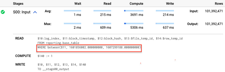
Note that you add the static filter to the staging table and keep T.block_timestamp = S.block_timestamp to convey to BigQuery that it can push that filter to the base table. This MERGE processes 41 GB of data in contrast to the initial 161 GB. You can see in the query plan that BigQuery pushes the partition filter from the staging table to the base table:
This type of optimization, when a pruning condition is pushed from a subquery to a large partitioned or clustered table, is not unique for MERGE. It also works for other types of queries. For instance:
SELECT * -- 41 GB processedFROM reporting.base_table TINNER JOIN staging.load_delta SON T.block_hash = S.block_hashAND T.log_index = S.log_indexAND T.block_timestamp = S.block_timestampWHERE S.block_timestamp BETWEEN TIMESTAMP '2020-10-05' AND TIMESTAMP '2020-12-07'
And you can check the query plan to verify that BigQuery pushed down the partition filter from one table to another.
Moreover, for SELECT statements, BigQuery can automatically infer a filter predicate on a join column and push it down from one table to another if your query meets the following criteria:
- The target table must be clustered or partitioned.
- The result size of the other table, i.e. after applying all filters, must qualify for broadcast join. Namly, the result set must be relatively small, less than ~100MB.
In our running example, reporting.base_table is partitioned by block_timestamp. If you define a selective filter on staging.load_delta and join two tables, you can see an inferred filter on the join key pushed to the target table
SELECT *FROM reporting.base_table TINNER JOIN staging.load_delta SON T.block_timestamp = S.block_timestampWHERE S.block_hash = '0x0c1caa16b34d94843aabfebc0d5a961db358135988f7498a6fdc450ad55f0870'
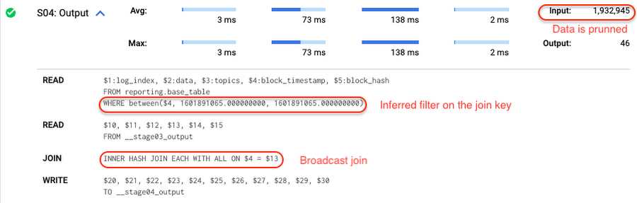
There is no requirement to join tables by partitioning or clustering key to kick off this type of optimization. However, in this case the pruning effect on the target table would be less significant.
But let us get back to the pipeline optimizations. Another way to enhance MERGE is to modify the merge_condition filter by adding static predicate on the base table:
BEGINDECLARE src_range STRUCT<date_min TIMESTAMP, date_max TIMESTAMP> --115 MB processedDEFAULT(SELECT STRUCT(MIN(block_timestamp) AS date_min,MAX(block_timestamp) AS date_max) FROM staging.load_delta);MERGE INTO reporting.base_table T --41 GB processedUSING staging.load_delta SON T.block_hash = S.block_hashAND T.log_index = S.log_indexAND T.block_timestamp BETWEEN src_range.date_min AND src_range.date_maxWHEN MATCHED THEN UPDATE SETT.data = S.dataWHEN NOT MATCHED THEN INSERT (log_index, data, topics, block_timestamp, block_hash)VALUES (log_index, data, topics, block_timestamp, block_hash);END;
To summarize, here are the steps that you can perform to enhance incremental ingestion pipelines in BigQuery. First you compute the range of updated partitions based on the small staging table. Next, you tweak the MERGE statement a bit to let BigQuery know to prune data in the base table.
All the enhanced MERGE statements scanned 41 GB of data, and setting up the src_range variable took 115 MB. Compare it with the initial 161 GB scan. Moreover, given that computing src_range may be incorporated into some existing transformation in your ETL/ELT, it results in a good performance improvement which you can leverage in your pipelines.
In this post we described how to enhance data ingestion pipelines by turning dynamic filter predicates into static predicates and letting BiQuery prune data for us. You can find more tips on BigQuery DML tuning here.
Special thanks to Daniel De Leo, who helped with examples and provided valuable feedback on this content.
HarbourBridge Schema Assistant Allows Quick, Bulk Migration to Cloud Spanner

5470
Of your peers have already read this article.
1:30 Minutes
The most insightful time you'll spend today!
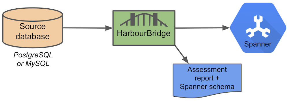
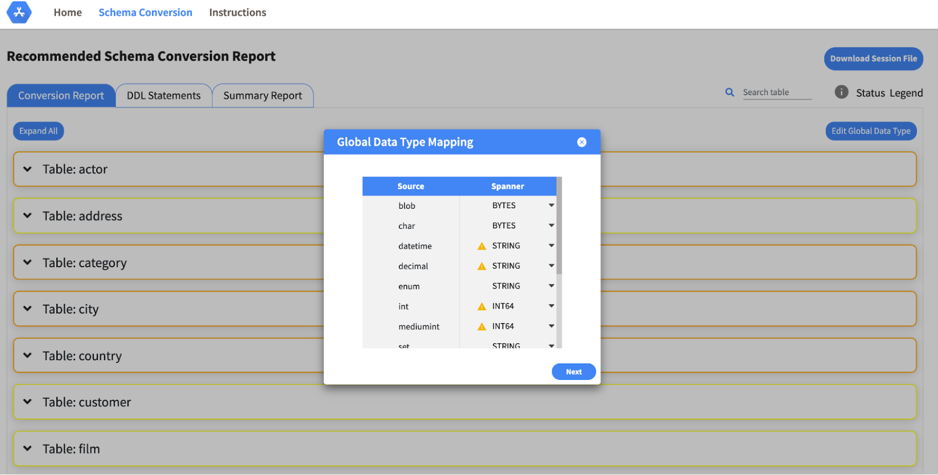
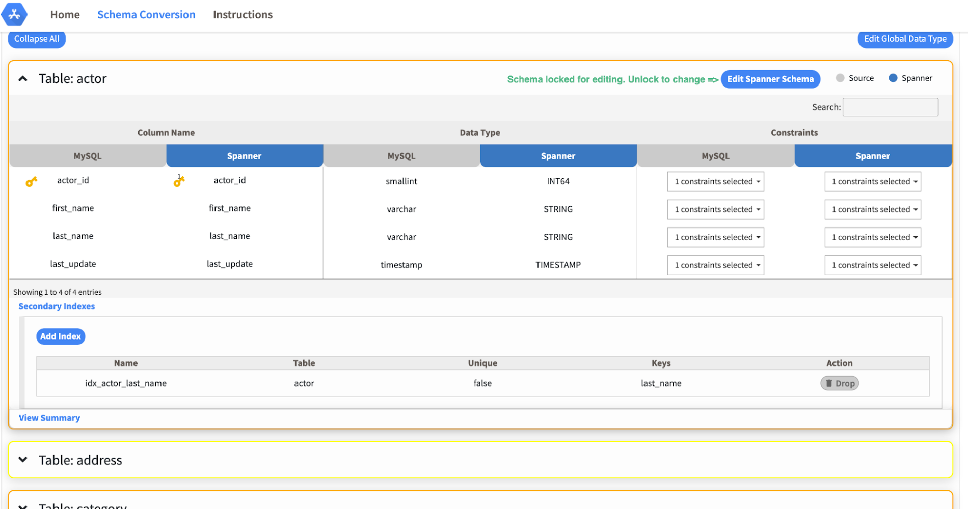
Today we’re announcing the HarbourBridge Schema Assistant, which provides a guided schema-design workflow for migrating from MySQL or PostgreSQL to Spanner. HarbourBridge imports dump files (from mysqldump or pg_dump) or directly connects to your source database, and converts the source database schema to an equivalent Spanner schema. The new Schema Assistant capability displays the source schema and Spanner schema side-by-side, highlights errors and walks you through a series of steps to validate and optimize your Spanner schema. It also produces a browsable assessment report with an overall migration-fitness score for Spanner, a table-by-table detailed analysis of type mappings and a list of features used in the source database that aren’t supported by Spanner. It supports editing of table and column names, column types, primary keys and constraints, as well as dropping of tables, columns, foreign keys and secondary indexes.
The new Schema Assistant complements HarbourBridge’s existing data and schema migration capabilities and is a critical step towards our goal of building a complete open-source migration toolkit. HarbourBridge continues to support command-line schema and data migration and turn-key Spanner evaluation.
Complementing the bulk data migration capabilities of HarbourBridge, we are also announcing the ability to migrate change events from MySQL to Cloud Spanner.
Supported Features in Schema Assistant
- Global type mapping. Users can customize the global mapping for how types should be mapped to Spanner consistently across the schema. For example, mapping large integers in source schema to Spanner’s NUMERIC.
- Local type mapping. Users can override the custom type mapping for a given table/column.
- Session management. A session keeps track of all the changes made to the schema mapping.
- Customization of secondary indexes. Users can add, edit and delete secondary indexes to optimize their Spanner performance.
- Customization of foreign keys and interleaved tables. Table interleaving is an important design consideration when migrating to Cloud Spanner as explained in more detail in this blog post.
Features in the pipeline
We are already working to further expand the supported set of schema editing features and welcome your feedback. We are particularly excited to expand the Schema Assistant’s design recommendations for optimizing Spanner schemas e.g. in-depth recommendations for primary key design.
HarbourBridge is open source and we gladly accept contributions from the wider community.
Transform ‘Dark Data’ from Documents with Document AI, Cloud Functions and Workflows

8201
Of your peers have already read this article.
2:00 Minutes
The most insightful time you'll spend today!
At enterprises across industries, documents are at the center of core business processes. Documents store a treasure trove of valuable information whether it’s a company’s invoices, HR documents, tax forms and much more. However, the unstructured nature of documents make them difficult to work with as a data source. We call this “dark data” or unstructured data that businesses collect, process and store but do not utilize for purposes such as analytics, monetization, etc. These documents in pdf or image formats, often trigger complex processes that have historically relied on fragmented technology and manual steps. With compute solutions on Google Cloud and Document AI, you can create seamless integrations and easy to use applications for your users. Document AI is a platform and a family of solutions that help businesses to transform documents into structured data backed by machine learning. In this blog post we’ll walk you through how to use Serverless technology to process documents with Cloud Functions, and with workflows of business processes orchestrating microservices, API calls, and functions, thanks to Workflows.
At Cloud Next 2021, we presented how to build easy AI-powered applications with Google Cloud. We introduced a sample application for handling incoming expense reports, analyzing expense receipts with Procurement Document AI, a DocAI solution for automating procurement data capture from forms including invoices, utility statements and more. Then organizing the logic of a report approval process with Workflows, and used Cloud Functions as glue to invoke the workflow, and do analysis of the parsed document.
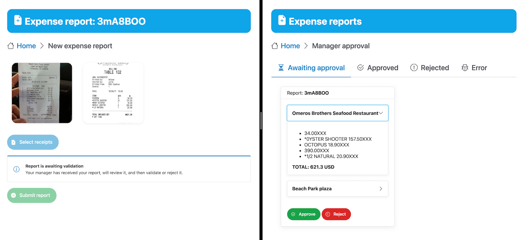
We also open sourced the code on this Github repository, if you’re interested in learning more about this application.
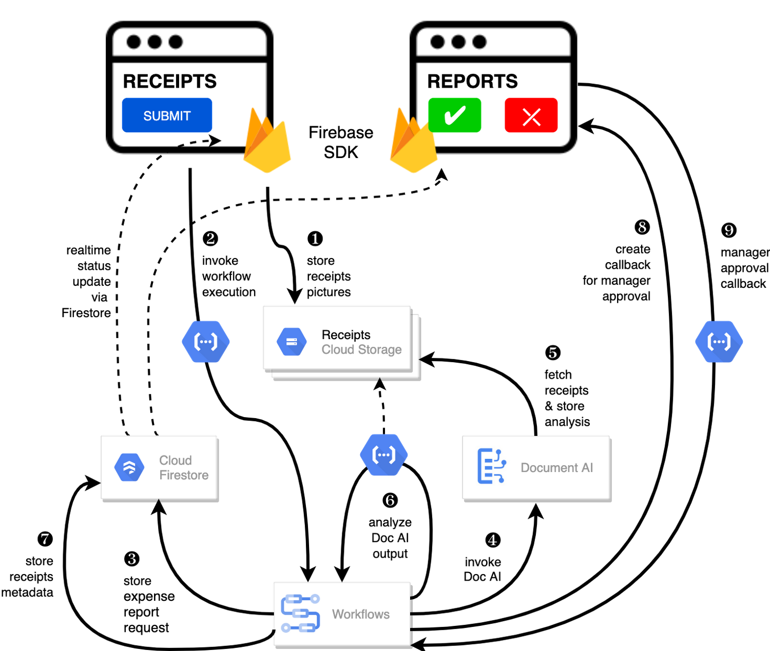
In the above diagram, there are two user journeys: the employee submitting an expense report where multiple receipts are processed at once, and the manager validating or rejecting the expense report.
First, the employee goes to the website, powered by Vue.js for the frontend progressive JavaScript framework and Shoelace for the library of web components. The website is hosted via Firebase Hosting. The frontend invokes an HTTP function that triggers the execution of our business workflow, defined using the Workflows YAML syntax.
Workflows is able to handle long-running operations without any additional code required, in our case we are asynchronously processing a set receipt files. Here, the Document AI connector directly calls the batch processing endpoint for service. This API returns a long-running operation: if you poll the API, the operation state will be “RUNNING” until it has reached a “SUCCEEDED” or “FAILED” state. You would have to wait for its completion. However, Workflows’ connectors handle such long-running operations, without you having to poll the API multiple times till the state changes. Here’s how we call the batch processing operation of the Document AI connector:
- invoke_document_ai:call: googleapis.documentai.v1.projects.locations.processors.batchProcessargs:name: ${"projects/" + project + "/locations/eu/processors/" + processorId}location: "eu"body:inputDocuments:gcsPrefix:gcsUriPrefix: ${bucket_input + report_id}documentOutputConfig:gcsOutputConfig:gcsUri: ${bucket_output + report_id}skipHumanReview: trueresult: document_ai_response
Machine learning uses state of the art Vision and Natural Language Processing models to intelligently extract schematized data from documents with Document AI. As a developer, you don’t have to figure out how to fine tune or reframe the receipt pictures, or how to find the relevant field and information in the receipt. It’s Document AI’s job to help you here: it will return a JSON document whose fields are: line_item, currency, supplier_name, total_amount, etc. Document AI is capable of understanding standardized papers and forms, including invoices, lending documents, pay slips, driver licenses, and more.
A cloud function retrieves all the relevant fields of the receipts, and makes its own tallies, before submitting the expense report for approval to the manager. Another useful feature of Workflows is put to good use: Callbacks, that we introduced last year. In the workflow definition we create a callback endpoint, and the workflow execution will wait for the callback to be called to continue its flow, thanks to those two instructions:
- create_callback:call: events.create_callback_endpointargs:http_callback_method: "POST"result: callback_details...- await_callback:try:call: events.await_callbackargs:callback: ${callback_details}timeout: 3600result: callback_requestexcept:as: esteps:- update_status_to_error:...
In this example application, we combined the intelligent capabilities of Document AI to transform complex image documents into usable structured data, with Cloud Functions for data transformation, process triggering, and callback handling logic, and Workflows enabled us to orchestrate the underlying business process and its service call logic.
Going further
If you’re looking to make sense of your documents, turning dark data into structured information, be sure to check out what Document AI offers. You can also get your hands on a codelab to get started quickly, in which you’ll get a chance at processing handwritten forms. If you want to explore Workflows, quickstarts are available to guide you through your first steps, and likewise, another codelab explores the basics of Workflows. As mentioned earlier, for a concrete example, the source code of our smart expense application is available on Github. Don’t hesitate to reach out to us at @glaforge and @asrivas_dev to discuss smart scalable apps with us.
6077
Of your peers have already watched this video.
1:30 Minutes
The most insightful time you'll spend today!
Explore the Innovations and Architecture Powering Spanner and BigQuery
Previously, databases had architectures with tightly coupled storage and compute. This resulted in higher latency, and with faster networks these constraints no longer surface. With Google Cloud’s BigQuery and CloudSpanner, the storage and compute architecture have been separated, allowing for better scalability and availability to address businesses’ high throughput data needs.
Watch the video to understand how these database and analysis products leverage Google’s distributed storage system, in-house custom network hardware and software, internal cluster management system and more!
More Relevant Stories for Your Company

Cloud IoT Core Helps Businesses Leverage their IoT Data to Build a Competitive Edge
The ability to gain real-time insights from IoT data can redefine competitiveness for businesses. Intelligence allows connected devices and assets to interact efficiently with applications and with human beings in an intuitive and non-disruptive way. After your IoT project is up and running, many devices will be producing lots of

Dataflow is getting better with Dataflow Prime, Dataflow Go, and Dataflow ML
By the end of 2024, 75% of enterprises will shift from piloting to operationalizing artificial intelligence according to IDC, yet the growing complexity of data types, heterogeneous data stacks and programming languages make this a challenge for all data engineers. With the current economic climate, doing more with cheaper costs

Brazilian Insurer Uses Google BigQuery to Underwrite Critical Decisions
To stay competitive in the rapidly changing insurance marketplace, Mitsui Sumitomo Seguros (MSS) recognized the need to leverage its available data to stabilize and scale existing operations, improve sales decisions and better engage employees. MSS managers required frequent and easy access to newly organized data (including performance metrics and market

BigQuery Explainable AI for Demystifying the Inner Workings of ML Models. Now GA!
Explainable AI (XAI) helps you understand and interpret how your machine learning models make decisions. We're excited to announce that BigQuery Explainable AI is now generally available (GA). BigQuery is the data warehouse that supports explainable AI in a most comprehensive way w.r.t both XAI methodology and model types. It does this at
