





Google Cloud CCAI’s Support for the Public Sector Soars during the Pandemic

5261
Of your peers have already read this article.
2:00 Minutes
The most insightful time you'll spend today!
Scaling Virtual Support in the Pandemic Era: The AI Connection
Since the early days of the pandemic, we’ve partnered with government organizations and academic institutions to serve communities at scale with Contact Center Artificial Intelligence (CCAI). I sat down with Bill MacKenzie, IT liaison for the Upper Grand School District in Ontario, and Marco Palermo, director of digital government and modernization, to discuss how they embraced CCAI to introduce scalable service delivery to residents and students alike. I’m sharing more on their stories below, and for the full overview, check out our Google Cloud Public Sector Summit session, Scaling Virtual Support in the Pandemic Era: The AI Connection.
Upper Grand School District: Answering questions with speed and accuracy
Bill MacKenzie described the Upper Grand School District’s struggles at the beginning of the pandemic, particularly helping parents with IT issues. The staff-oriented help desk was not equipped to assist parents trying to securely login for students as young as kindergarten. Without sufficient support for parents, the District was struggling to handle thousands of phone calls a day.
To alleviate the manual strain, they turned to Quantiphi, a Google Cloud partner, to implement Google Cloud Dialogflow. They were fully functional within a few weeks. The new website provided real-time responses as well as clear documentation to help parents get up and running quickly.
“In the first 10 days, we had over 5,000 hits, and the accuracy rate was 92%,” MacKenzie said.
The district doesn’t know what the future holds, but now that they have been through the process, they are confident they now understand how to create their own bots to meet critical needs.
City of Toronto: Getting critical information to the community
Marco Palermo explained how the city of Toronto was facing a very rapid and fluid situation at the beginning of the pandemic. Getting information to constituents was extremely important, and they needed alternative channels to deliver that information.
Toronto has been committed to workforce equity and inclusivity in order to best represent the diversity of its residents. As a result, solutions had to be accessible to all. The bot handled 25,330 unique users and addressed 20,174 total questions with an 80% accurate response rate in the first four months. It’s been a huge success for the city, with plans to expand its capabilities.
Personalized response to the pandemic challenge
I noted that even before the pandemic, government leaders were asking for a way to provide more flexible personal experiences and better support outside of normal business hours. Around 60% of constituents want more self-service options and 75% would happily interact with digital resources if they could get the answers they needed.
Google Cloud CCAI addresses these needs with a single core of intelligence that provides a consistently high-quality conversational experience—human or virtual—across all channels and platforms. It can be deployed on legacy infrastructure without upgrades in an average of two weeks.
CCAI operates with a conversational core that centralizes the ability to talk, understand, and interact, orchestrating high-quality conversations at scale. It provides services in three different ways:
- Virtual Agent AI allows natural conversation with customers to identify and address their issues effectively
- Agent Assist AI helps human agents by providing real-time turn-by-turn guidance so they can better serve constituents
- Insight AI determines metrics and trends in real-time to enable faster and more accurate insights
CCAI provides consistency across every application. It can go off-script when answering complex questions, adjusting human conversation with the capacity to handle unexpected stops and starts, odd word choices, or implied meanings. It can also handle multiple use cases for the customer, such as taking payments, updating information, providing information, and more. By allowing agencies to automate routine tasks and reduce the amount of time employees need to dedicate to answering calls, the solution created cost savings for the agency.
Explore more on this session by visiting the Public Sector Summit on-demand video.
Leverage ML to Spot Anomalies in Real-time Forex Data

3100
Of your peers have already read this article.
6:00 Minutes
The most insightful time you'll spend today!
Let’s say you are a quantitative trader with access to real-time foreign exchange (forex) price data from your favorite market data provider. Perhaps you have a data partner subscription, or you’re using a synthetic data generator to prove value first. You know there must be thousands of other quants out there with your same goal. How will you differentiate your anomaly detector?
What if, instead of training an anomaly detector on raw forex price data, you detected anomalies in an indicator that already provides generally agreed buy and sell signals? Relative Strength Index (RSI) is one such indicator; it is often said that RSI going above 70 is a sell signal, and RSI going below 30 is a buy signal. As this is just a simplified rule, it means there could be times when the signal is inaccurate, such as a currency market correction, making it a prime opportunity for an anomaly detector.
This gives us the following high level components:

Of course, we want each of these components to handle data in real time, and scale elastically as needed. Dataflow pipelines and Pub/Sub are the perfect services for this. All we need to do is write our components on top of the Apache Beam sdk, and they’ll have the benefit of distributed, resilient and scalable compute.
Luckily for us, there are some great existing Google plugins for Apache Beam. Namely, a Dataflow time-series sample library that includes RSI calculations, and a lot of other useful time series metrics; and a connector for using AI Platform or Vertex AI inference within a Dataflow pipeline. Let’s update our diagram to match, where the solid arrows represent Pub/Sub topics.
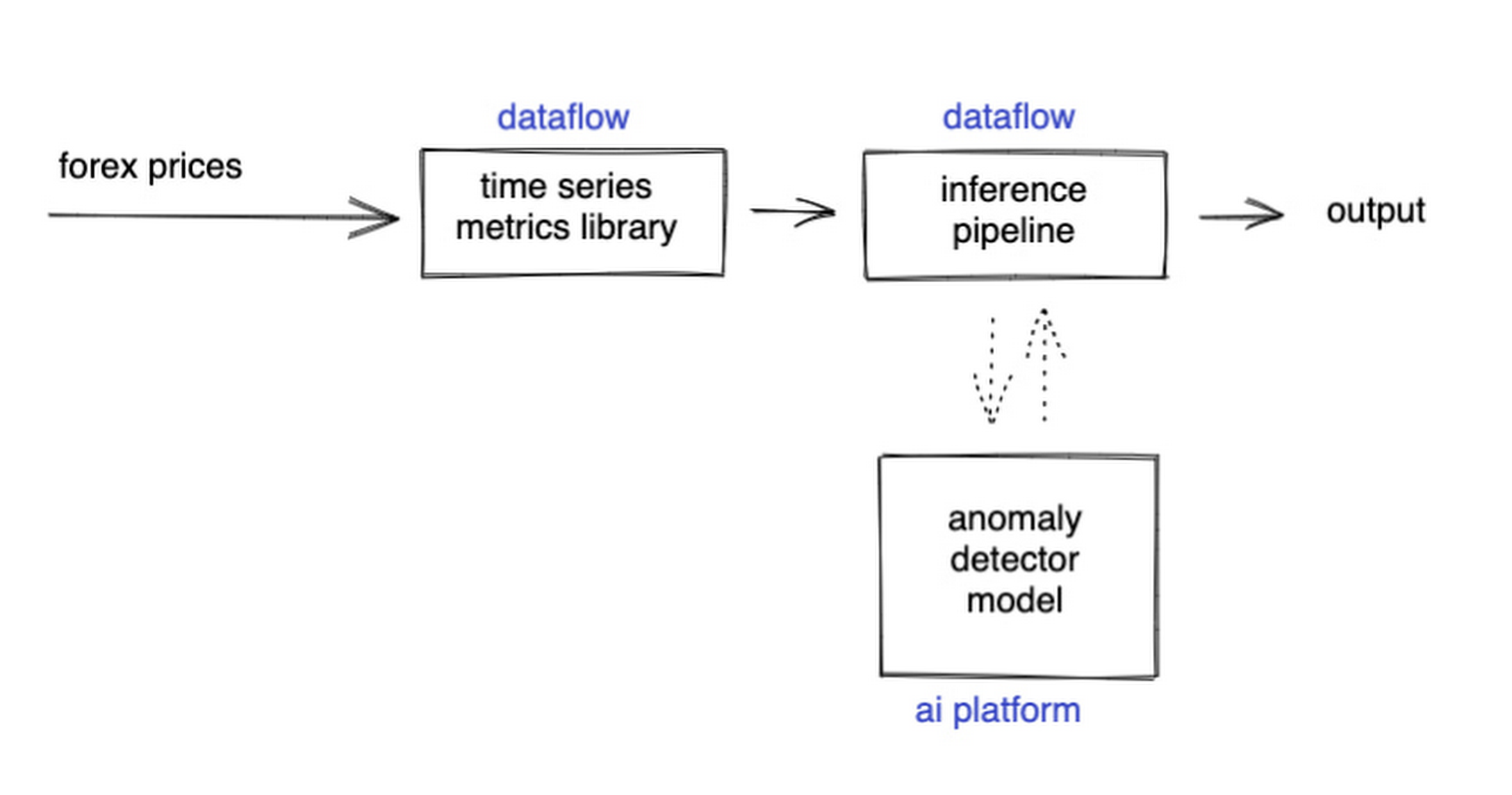
The Dataflow time-series sample library also provides us with gap-filling capabilities, which means we can rely on having contiguous data once the flow reaches our machine learning (ML) model. This lets us implement quite complex ML models, and means we have one less edge case to worry about.
So far we’ve only talked about the real time data flow, but for visualization and continuous retraining of our ML model, we’re going to want historical data as well. Let’s use BigQuery as our data warehouse, and Dataflow to plumb Pub/Sub into it. As this plumbing job is embarrassingly parallelizable, we wrote our pipeline to be generic across data types and share the same Dataflow job, such that compute resources can be shared. This results in efficiencies of scale both in cost savings and time required to scale-up.

Data Modeling
Let’s discuss data formats a bit further here. An important aspect of running any data engineering project at scale is flexibility, interoperability and ease of debugging. As such, we opted to use flat JSON structures for each of our data types, because they are human readable and ubiquitously understood by tooling. As BigQuery understands them too, it’s easy to jump into the BigQuery console and confirm each component of the project is working as expected.
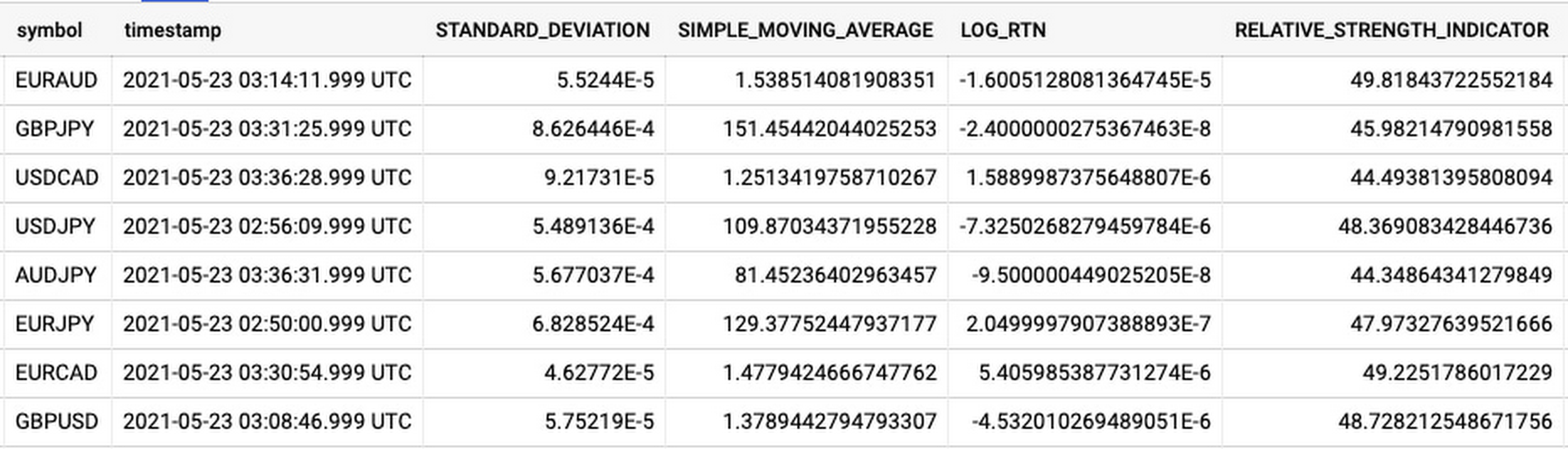
As you can see, the Dataflow sample library is able to generate many more metrics than RSI. It supports generating two types of metrics across time series windows, metrics which can be calculated on unordered windows, and metrics which require ordered windows, which the library refers to as Type 1 metrics and Type 2 metrics, respectively. Unordered metrics have a many-to-one relationship, which can help reduce the size of your data by reducing the frequency of points through time. Ordered metrics run on the outputs of the unordered metrics, and help to spread information through the time domain without loss in resolution. Be sure to check out the Dataflow sample library documentation for a comprehensive list of metrics supported out of the box.
As our output is going to be interpreted by our human quant, let’s use the unordered metrics to reduce the time resolution of our flow of real time data to one per second, or one hertz. If our output was being passed into an automated trading algorithm, we might choose a higher frequency. The decision for the size of our ordered metrics window is a little more difficult, but broadly determines the amount of time-steps our ML model will have for context, and therefore the window of time for which our anomaly detection will be relevant. We at least need it to be larger than our end-to-end latency, to ensure our quant will have time to act. Let’s set it to five minutes.
Data Visualization
Before we dive into our ML model, let’s work on visualization to give us a more intuitive feel for what’s happening with the metrics, and confirm everything we’ve got so far is working. We use the Grafana helm chart with the BigQuery plugin on a Google Kubernetes Engine (GKE) Autopilot cluster. The visualisation setup is entirely config-driven and provides out-of-the-box scaling, and GKE gives us a place to host some other components later on.
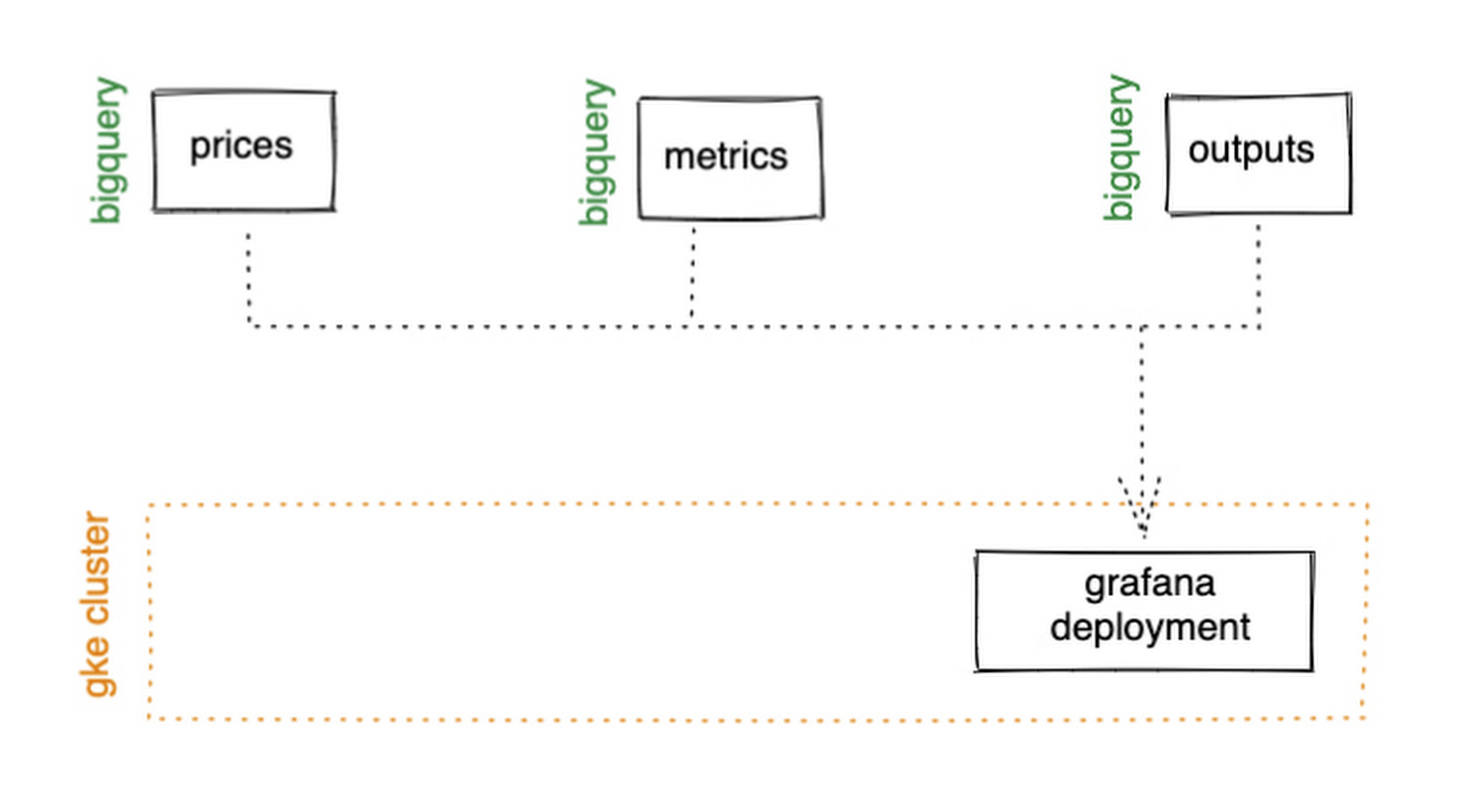
GKE Autopilot has Workload Identity enabled by default, which means we don’t need to worry about passing around secrets for BigQuery access, and can instead just create a GCP service account that has read access to BigQuery and assign it to our deployment through the linked Kubernetes service account.
That’s it! We can now create some panels in a Grafana dashboard and see the gap filling and metrics working in real time.

Building and deploying the Machine Learning Model
Ok, ML time. As we alluded to earlier, we want to continuously retrain our ML model as new data becomes available, to ensure it remains up to date with the current trend of the market. TensorFlow Extended (TFX) is a platform for creating end-to-end machine learning pipelines in production, and eases the process around building a reusable training pipeline. It also has extensions for publishing to AI Platform or Vertex AI, and it can use Dataflow runners, which makes it a good fit for our architecture. The TFX pipeline still needs an orchestrator, so we can host that in a Kubernetes job, and if we wrap it in a scheduled job, then our retraining happens on a schedule too!

TFX requires our data be in the tf.Example format. The Dataflow sample library can output tf.Examples directly, but this tightly couples our two pipelines together. If we want to be able to run multiple ML models in parallel, or train new models on existing historical data, we need our pipelines to only be loosely coupled. Another option is to use the default TFX BigQuery adaptor, but this restricts us to each row in BigQuery mapping to exactly one ML sample, meaning we can’t use recurrent networks.
As neither of the out-of-the-box solutions met our requirements, we decided to write a custom TFX component that did what we needed. Our custom TFX BigQuery adaptor enables us to keep our standard JSON data format in BigQuery and train recurrent networks, and it keeps our pipelines loosely coupled! We need the windowing logic to be the same for both training and inference time, so we built our custom TFX component using standard Beam components, such that the same code can be imported in both pipelines.
def window_elements(pipeline: beam.Pipeline,window_length: int,drop_irregular_windows: bool = True,sort_windows_by: str = "timestamp",):"""Window elements into regular windows of a given size.Assumes elements flow at a fixed rate of 1Hz."""def _sort_windows(window: Iterable[Dict[Text, Any]]) -> List[Dict[Text, Any]]:sorted_window = sorted(window, key=lambda e: e[sort_windows_by])return sorted_windowwindowed_elements = (pipeline| "AddConstantKey" >> beam.Map(lambda item: (0, item))| "WithSlidingWindow">> beam.WindowInto(beam.transforms.window.SlidingWindows(window_length, 1),trigger=beam.transforms.trigger.AfterCount(window_length),accumulation_mode=beam.transforms.trigger.AccumulationMode.DISCARDING,)| "CombineWindow" >> beam.GroupByKey()| "GetValues" >> beam.Values())if drop_irregular_windows:windowed_elements = windowed_elements | "EnforceWindowLengths" >> beam.Filter(lambda w: len(w) == window_length).with_output_types(List[Dict[Text, Any]])if sort_windows_by is not None:windowed_elements = windowed_elements | "Sort" >> beam.Map(_sort_windows).with_output_types(List[Dict[Text, Any]])return windowed_elements
With our custom generator done, we can start designing our anomaly detection model. An autoencoder utilising long-short-term-memory (LSTM) is a good fit for our time-series use case. The autoencoder will try to reconstruct the sample input data, and we can then measure how close it gets. That difference is known as the reconstruction error. If there is a large enough error, we call that sample an anomaly. To learn more about autoencoders, please consider reading chapter 14 from Deep Learning by Ian Goodfellow, Yoshua Bengio, and Aaron Courville.
Our model uses simple moving average, exponential moving average, standard deviation, and log returns as input and output features. For both the encoder and decoder subnetworks, we have 2 layers of 30 time step LSTMs, with 32 and 16 neurons, respectively.
In our training pipeline, we include z score scaling as a preprocessing transformer – which is usually a good idea when it comes to ML. However, there’s a nuance to using an autoencoder for anomaly detection. We need not only the output of the model, but also the input, in order to calculate the reconstruction error. We’re able to do this by using model serving functions to ensure our model returns both the output and preprocessed input as part of its response. As TFX has out-of-the-box support for pushing trained models to AI Platform, all we need to do is configure the pusher, and our (re)training component is complete.
Detecting Anomalies in real time
Now that we have our model in Google Cloud AI Platform, we need our inference pipeline to call to it in real time. As our data is using standard JSON, we can easily apply our RSI rule of thumb inline, ensuring our model only runs when needed. Using the reconstructed output from AI Platform, we are then able to calculate the reconstruction error. We choose to stream this directly into Pub/Sub to enable us to dynamically apply an anomaly threshold when visualising, but if you had a static threshold you could apply it here too.
with beam.Pipeline(options=pipeline_options) as pipeline:(pipeline| "ReadFromPubSub">> beam.io.ReadFromPubSub(topic=input_metrics,timestamp_attribute=timestamp_key,)| "DeserialiseJSON" >> beam.Map(pubsub_serialiser.to_json)| "FilterSymbol" >> beam.Filter(lambda m: m["symbol"] == symbol)| "FilterRSIThreshold">> beam.Filter(lambda m: m["RELATIVE_STRENGTH_INDICATOR"] > rsi_upper_thresholdor m["RELATIVE_STRENGTH_INDICATOR"] < rsi_lower_threshold)| "WindowElements" >> window_elements(window_length)| "RunAutoencoder">> run_windowed_inference(gcp_project_id,model_name,window_length,{f: "FLOAT" for f in feature_metrics},)| "CalcReconError" >> beam.Map(calc_reconstruction_err)| "ToJSON">> beam.Map(lambda re: {"symbol": symbol, "reconstruction_error": re})| "SerialiseJSON" >> beam.Map(pubsub_serialiser.from_json)| "WriteToPubSub">> beam.io.WriteToPubSub(topic=output_alerts,timestamp_attribute=timestamp_key,))
Summary
Here’s what the wider architecture looks like now:

More importantly though, does it fit for our use case? We can plot the reconstruction error of our anomaly detector against the standard RSI buy/sell signal, and see when our model is telling us that perhaps we shouldn’t blindly trust our rule of thumb. Go get ‘em, quant!
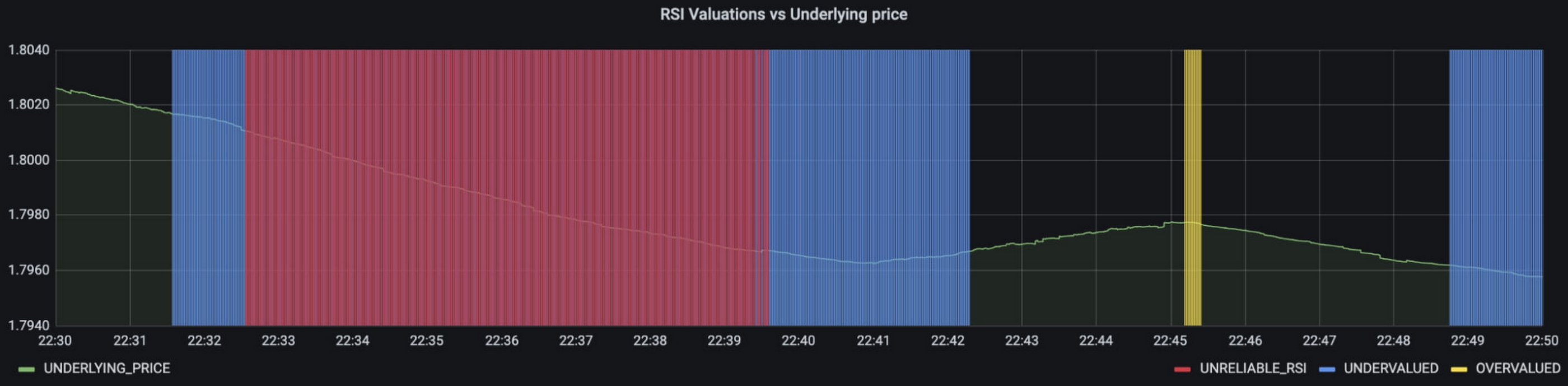
In terms of next steps, there are many things you could do to extend or adapt what we’ve covered. You might want to explore with multi-currency models, where you could detect when the price action of correlated currencies is unexpected, or you could connect all of the Pub/Sub topics to a visualization tool to provide a real-time dashboard.
Give it a try
To finish it all off, and to enable you to clone the repo and set everything up in your own environment, we include a data synthesizer to generate forex data without needing access to a real exchange. As you might have guessed, we host this on our GKE cluster as well. There are a lot of other moving parts – TFX uses a SQL database and all of the application code is packaged into a docker image and deployed along with the infra using Terraform and cloud build. But if you’re interested in those nitty gritty details, head over to the repo and get cloning!
Feel free to reach out to our teams at Google Cloud and Kasna for help in making this pattern work best for your company.
Guide to Create and Manage Datasets with Vertex AI

3046
Of your peers have already read this article.
2:00 Minutes
The most insightful time you'll spend today!
At Google I/O this year, we introduced Vertex AI to bring together all our ML offerings into a single environment that lets you build and manage the lifecycle of ML projects. In a previous post, we gave you an overview of Vertex AI, sharing how it supports your entire ML workflow—from data management all the way to predictions. Today, we’ll talk a little about how to manage ML datasets with Vertex AI.
Many enterprises want to use data to make meaningful predictions that can bolster their business or help them venture into new markets. This often requires using custom machine learning models—something not every business knows how to create or use. This is where Vertex AI can help. Vertex AI provides tools for every step of the machine learning workflow—from managing data sets to different ways of training the model, evaluating, deploying, and making predictions. It also supports varying levels of ML expertise, so you don’t need to be an ML expert to use Vertex AI.https://www.youtube.com/embed/CN2X6oIlnmI?enablejsapi=1&
Types of data you can use in Vertex AI
Datasets are the first step of the machine learning lifecycle—to get started you need data, and lots of it. Vertex AI currently supports managed datasets for four data types—image, tabular, text, and videos.
Image
Image datasets let you do:
- Image classification—Identifying items within an image.
- Object detection—Identifying the location of an item in an image
- Image segmentation—Assigning labels to pixel level regions in an image.
To ensure your model performs well in production, use training images similar to what your users will send. For example, if users are likely to send low quality images, be sure to have blurry and low resolution images in your data set. Don’t forget to include different angles, backgrounds, and resolutions. We recommend you include at least 1,000 images per label (item you want to identify), but you can always get started with 10 per label. The more examples you provide, the better your model will be.
Tabular
Tabular datasets enable you to do:
- Regression—Predicting a numerical value.
- Classification—Predicting a category associated with a particular example.
- Forecasting—Predicting the likelihood of sudden events or demands.
Tabular data sets support hundreds of columns and millions of rows.
Text
With text datasets, you can do:
- Classification—Assigning one or more labels to an entire document.
- Entity extraction—Identifying custom text entities within a document, like “too expensive” or “great value”.
- Sentiment analysis—Identifying the overall sentiment expressed in a block of text, for example, if a customer was happy or upset or frustrated.
Video
Video datasets enable:
- Classification—Labeling entire videos, shots, or frames.
- Action recognition—Identifying clips video clips where specific actions occur.
- Object tracking—Tracking specific objects in a video.
Creating and managing datasets in Vertex AI
Now that we’ve covered the different types of data you can use, let’s shift to creating and managing those datasets. In the Cloud Console, go to Vertex AI dashboard page and click Datasets, then click Create Project.
Say you want to classify items within a set of photos. Create an image dataset and select image classification. You can import files directly from your computer, which will be stored in Cloud Storage. Then, you’ll need to add the corresponding labels (items you want to identify) for your images. If you already have labels, you can use the Import File option to import a CSV with your image URLs and their labels. If your data is not labeled and you would like human help to label it, you can use the Vertex AI data labeling service. Once the files are uploaded, you can create labels and assign them to the images. You can also analyze the images in the data set, the number of images per label, and a few other properties.
Depending on the type of data you use, your options might vary slightly. For example, if you want to use tabular data, you could upload a CSV file from your computer, use one from Cloud Storage, or select a table from BigQuery directly. Once you select the table, the data is available for analysis.
More to come
This concludes our overview of creating and managing datasets in Vertex AI. In a future installment, we’ll go over the next phase of the machine learning workflow: building and training ML models.
If you enjoyed this post, keep an eye out for more AI Simplified episodes on YouTube. In the meantime, here’s where you can learn more about Vertex AI.
Canadian Bank’s SAP Workload Moved to BigQuery Helps Unlock New Business Opportunities

7341
Of your peers have already read this article.
2:00 Minutes
The most insightful time you'll spend today!
When ATB Financial decided to migrate its vast SAP landscape to the cloud, the primary goal was to focus on things that matter to customers as opposed to IT infrastructure. Based in Alberta, Canada, ATB Financial serves over 800,000 customers through hundreds of branches as well as digital banking options. To keep pace with competition from large banks and FinTech startups and to meet the increasing 24/7 demands of customers, digital transformation was a must. To support this new mandate, in 2019, ATB migrated its extensive SAP backbone to Google Cloud. In addition to SAP S/4 HANA, ATB runs SAP financial services, core banking, payment engine, CRM and business warehouse on Google Cloud.
In parallel, changes were needed to ATB’s legacy data platform. The platform had stability and reliability issues and also suffered from a lack of historical data governance. Analytics processes were ad hoc and manual. The legacy data environment was also not set up to tackle future business requirements that come with a high dependency on real-time data analysis and insights.
After evaluating several potential solutions, ATB chose BigQuery as a serverless data warehouse and data lake for its next-generation, cloud-native architecture. “BigQuery is a core component of what we call our data exposure enablement platform, or DEEP,” explains Dan Semmens, Head of Data and AI at ATB Financial. According to Semmens, DEEP consists of four pillars, all of which depend on Google Cloud and BigQuery to be successful:
- Real-time data acquisition: ATB uses BigQuery throughout its data pipeline, starting with sourcing, processing, and preparation, moving along to storage and organization, then discovery and access, and finally consumption and servicing. So far, ATB has ingested and classified 80% of its core SAP banking data as well as data from a number of its third-party partners, such as its treasury and cash management platform provider, its credit card provider, and its call center software.
- Data enrichment: Before migrating to Google Cloud, ATB managed a number of disconnected technologies that made data consolidation difficult. The legacy environment could handle only structured data, whereas Google Cloud and BigQuery lets the bank incorporate unstructured data sets, including sensor data, social network activity, voice, text, and images. ATB’s data enrichment program has enabled more than 160 of the bank’s top-priority insights running on BigQuery, including credit health decision models, financial reporting, and forecasting, as well as operational reporting for departments across the organization. Jobs such as marketing campaigns and month-end processes that used to take five to eight hours now run in seconds, saving over CA$2.24 million in productivity.
- Self-service analytics: Data for self-service reporting, dashboarding, and visualization is now available for ATB’s 400+ business users and data analysts. Previously, bringing data and analytics to the business users who needed it while ensuring security was burdensome for IT, fraught with recurrent data preparation and other highly manual elements. Now, ATB automates much of its data protection and governance controls through the entire data lifecycle management process. Data access is not only open to more team members but it is faster and easier to acquire without compromising security. And it’s not just raw data that users can access. ATB uses BigQuery to define its enterprise data models and create what it calls its data service layer to make it easier for team members to visualize their data.
- AI-assisted analytics and automation: Through Google Cloud and BigQuery, ATB has been able to publish data and ML models that provide alerts and notifications via APIs to customer service agents. These real-time recommendations allow customer service agents to provide more tailored service with contextualized advice and suggested new services. So far, the company has deployed more than 40 ML models to generate over 20,000 AI-assisted conversations per month. Thanks to improved customer advocacy and less churn, the bank has realized more than CA$4 million in operating revenue. During the ongoing COVID crisis, the system was also able to predict when business and personal banking customers were experiencing financial distress so that a relationship manager could proactively reach out to offer support, such as payment deferral or loan restructuring. The AI tools provided by BigQuery are also helping ATB detect fraud that previously evaded rules-based fraud detection by using broader sets of timely and accurate data.
Thanks to the speed and ease of moving data from SAP to BigQuery, ATB is using artificial intelligence (AI) and machine learning (ML) to do things it previously hadn’t thought possible, including sophisticated fraud prevention models, product recommendations, and enriched CRM data that improves the customer experience.
Using the power of Google Cloud and BigQuery, ATB Financial has been able to draw more value from its SAP data while lowering cost and improving security and reliability. Speed to provide data sets and insights to internal team members has improved 30%. The bank also has seen a 15x reduction in performance incidents while improving data governance and security. Dan Semmens projects that the digital transformation strategy built on Google Cloud and BigQuery has both saved millions compared to its on-premises environment and has also realized millions in new business opportunities.
Semmens is looking toward the future that includes initiatives like Open Banking and greater ability to provide real time personalized advice for customers to drive revenue growth. “We see our data platform as foundational to ATB’s 10-year strategy,” he says. “The work we’ve undertaken over the past 18 months has enabled critical functionality for that future.”
Learn more about how ATB Financial is leveraging BigQuery to gain more from SAP data. Visit us here to explore how Google Cloud, BigQuery, and other tools can unlock the full value of your SAP enterprise data.
How Google Cloud’s Scalable Data Storage and High Compute Resources Fuel Investment Research
6287
Of your peers have already read this article.
1:30 Minutes
The most insightful time you'll spend today!
Investment management is a heavily data-driven industry—portfolio managers and investment researchers require a large number of data sources to guide them in shaping their investment strategies.
New cloud capabilities and technologies enable investment managers to process data faster than ever before and iterate on ideas quickly to fuel innovation in the signal generation process and gain a competitive edge.
Using the cloud for investment research workflows makes it easier to onboard data from data providers, spin up large compute workloads in the midst of market volatility or during heavy research cycles, and manage complex machine learning or natural language workflows to gain market insights.
We hear from industry leaders that they’re exploring new ways to run investment research. “Differentiated investment strategies require new types of information sources, and new ways to process that information,” David Easthope, senior analyst, Market Structure and Technology, Greenwich Associates. “And that, of course, relies heavily on having access to reliable and scalable storage, computational, and AI / ML resources. More specifically, quantitative strategies can benefit from the computational platforms and embedded AI/ML capabilities the cloud can offer.”
Google Cloud gives investment managers essential components to work and operate faster as they bring their investment research workflows to the cloud. Here are the key highlights:
1. Simplify, speed up your data acquisition, discovery, and analytics
The foundation of any investment strategy starts with data—acquiring it, detecting patterns, and analyzing it for insights. Enabling data providers to easily share large datasets such as tick history within a high-performance analytics engine can greatly reduce the data engineering overhead when possible.
Once data is onboarded, you can tag business and technical metadata related to your datasets and provide portfolio managers the ability to discover these datasets via a search interface.
We further review analytics options for various scenarios, including aggregating massive datasets, creating dashboards, and incorporating streaming analytics workloads.
2. Take advantage of burst compute workloads
Data engineers and researchers require ready access to burst compute capabilities to perform backtesting, portfolio simulations and run risk calculations. Cloud works well for these workloads due to its elasticity, consumption-based models, and hardware evolution.
Many investment managers are shifting to a container-based strategy along with a Kubernetes-based scheduler for greater consistency, scaling and efficiency in environments with a large number of researchers. Cloud managed services and a rich suite of CI/CD tools can make this vision a reality while improving security and developer productivity.
3. Tackle machine learning (ML) and model deployment with the help from cloud
Quantitative researchers scour vast amounts of market and alternative data sources searching for signals and correlations, while ML engineers have the challenge of taking these signals and moving them to production.
Google Cloud empowers users to create and operationalize their models without wasting valuable time with a comprehensive set of MLOps tools.
In this paper, we explore multiple solutions for ML and model deployment. Those capabilities reduce the amount of time operationalizing ML models, so quants and data scientists have more time to devote to differentiating activities.
4. Get the data you need in less time with Natural Language and Document AI
Thousands of financial filings, news articles, and sell-side research reports are generated every day, and it’s difficult for humans alone to process this volume of information. These documents are often generated in many languages and the ability to do entity recognition, sentiment or syntactical analysis in those languages, or perhaps translate them into the language of the portfolio manager is of critical importance. Google Cloud provides these capabilities through pre-trained models, or allows you to train high-quality models with your own datasets.
Getting started
There are plenty of emerging technologies, tools, and approaches available to help investment managers today. At Google Cloud, we can help you access, organize, and utilize these essential components to make your research faster, reliable, and more valuable.
To learn more about these four keys to better investment research, check out our whitepaper for more.
ML Workflow Made Simple: How to Automate ML Experiment Tracking with Vertex AI Experiments Autologging

1255
Of your peers have already read this article.
3:30 Minutes
The most insightful time you'll spend today!
Practical machine learning (ML) is a trial and error process. ML practitioners compare different performance metrics by running ML experiments till you find the best model with a given set of parameters. Because of the experimental nature of ML, there are many reasons for tracking ML experiments and making them reproducible including debugging and compliance.
But tracking experiments is challenging: you need to organize experiments so that other team members can quickly understand, reproduce and compare them. That adds overhead that you don’t need.
We are happy to announce Vertex AI Experiments autologging, a solution which provides automated experiment tracking for your models, which streamlines your ML experimentation
With Vertex AI Experiments autologging, you can now log parameters, performance metrics and lineage artifacts by adding one line of code to your training script without needing to explicitly call any other logging methods.
How to use Vertex AI autologging
As a data scientist or ML practitioner, you conduct your experiment in a notebook environment such as Colab or Vertex AI Workbench. To enable Vertex AI Experiments autologging, you call aiplatform.autolog() in your Vertex AI Experiment session. After that call, any parameters, metrics and artifacts associated with model training are automatically logged and then accessible within the Vertex AI Experiment console.
Here’s how to enable autologging in your training session with a Scikit-learn model.
# Enable autologging
aiplatform.autolog()

# Build training pipeline
ml_pipeline = Pipeline(...)

# Train model
ml_pipeline.fit(x_train, y_train)
This video shows parameters and training/post-training metrics in the Vertex AI Experiment console.
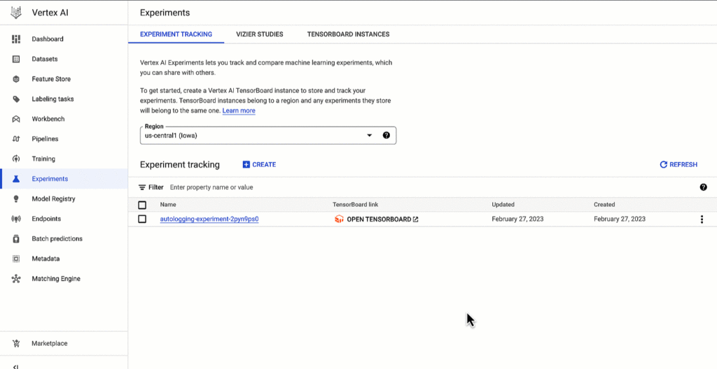
Vertex AI SDK autologging uses MLFlow’s autologging in its implementation and it supports several frameworks including XGBoost, Keras and Pytorch Lighting. See documentation for all supported frameworks.
Vertex AI Experiments autologging automatically logs model time series metrics when you train models along multiple epochs. That’s because of the integration between Vertex AI Experiments autologging and Vertex AI Tensorboard.
Furthermore, you can adapt Vertex AI Experiments autologging to your needs. For example, let’s say your team has a specific experiment naming convention. By default, Vertex AI Experiments autologging automatically creates Experiment Runs for you without requiring you to call `aiplatform.start_run()` or `aiplatform.end_run()`. If you’d like to specify your own Experiment Run names for autologging, you can manually initialize a specific run within the experiment using aiplatform.start_run() and aiplatform.end_run() after autologging has been enabled.
What’s next
You can access Vertex AI Experiments autologging with the latest version of Vertex AI SDK for Python. To learn more, check out these resources :
- Documentation: Autolog data to an experiment run
- Github: Get started with Vertex AI Experiments autologging
While I’m thinking about the next blog post, let me know if there is Vertex AI content you’d like to see on Linkedin or Twitter.
More Relevant Stories for Your Company




Navigating the AI Landscape: The Future of AI for ML Engineers
A podcast-style video series exploring how AI is shaping our future and how to prepare for changes. Developer advocate, Arwen Hauzhenga, shares his 10+ years of experience in machine learning and generative AI. He discusses the evolution of the field from data mining to data science and large-scale machine learning.

Geospatial Data for Business Apps Drive Sustainable and Accurate Decision-making
Organizations that collect geospatial data can use that information to understand their operations, help make better business decisions, and power innovation. Traditionally, organizations have required deep GIS expertise and tooling in order to deliver geospatial insights. In this post, we outline some ways that geospatial data can be used in

Driving Business Transformation in Healthcare Using Google Cloud and AI/ML
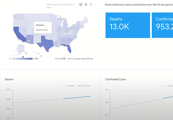
Before the COVID-19 pandemic, when you thought of healthcare and AI, a number of ideas sprang to mind. But the world, especially as it relates to healthcare has seen a completely different type of transformation as a result of COVID-19. This video is about how Google Cloud is helping organizations

Supercharge Marketing with Ready-Made, Centralized Smart Analytics
Your company has lots of valuable marketing data, but it’s spread across many systems and teams. That's a problem. In fact, only 13% of organisations feel like they're making the most out of their available customer data today. And the reason is that data--marketing and customer data--is spread across many
