





Architecting Multi-region Database Disaster Recovery for MySQL

4096
Of your peers have already read this article.
4:30 Minutes
The most insightful time you'll spend today!
Enterprises expect extreme reliability of the database infrastructure that’s accessed by their applications. Despite your best intentions and careful engineering, database errors happen, whether that’s machine crashes or network partitioning. Good planning can help you stay ahead of problems and recover more quickly when issues do occur.
This blog shows one approach of deploying a database architecture that implements high availability and disaster recovery for MySQL on Compute Engine, using regional disks as well as load balancers.
Any database architecture must provide approaches to tolerate errors and recover from those errors quickly without losing data. These approaches are expressed in RTO (recovery time objective) and RPO (recovery point objective), which offer ways to set and then measure how long a service can be unavailable, and how far back data should be saved.
After a database error, a database must recover as fast as possible with an RTO as small as possible, ideally in seconds. There must be as little data loss as possible—ideally, none at all. The desired RPO is the last consistent database state.
From a database architecture and deployment viewpoint, this can be accomplished with two distinct concepts: high availability and disaster recovery. Use both at the same time in order to achieve an architecture that’s prepared for the widest range of errors or incidents.
Creating a resilient database architecture
A high-availability database architecture has database instances in two or more zones. If a server on a zone fails, or the zone becomes inaccessible, the instances in other zones are available to continue the processing. The figure below shows two instances, one in zone zn1, and one in zone zn2. The load balancer in front supports directing traffic to a healthy database instance available for read and write queries.
A disaster recovery architecture adds a second high-availability database setup in a second region. If one of the regions becomes inaccessible or fails, the other region takes over. The figure below shows two regions, primary and DR. Data is replicated from the primary to the DR region so that the DR region can take over from the latest consistent database state. The load balancer in front of the regions directs traffic to the region in charge of the read and write traffic. Here’s how this architecture looks:
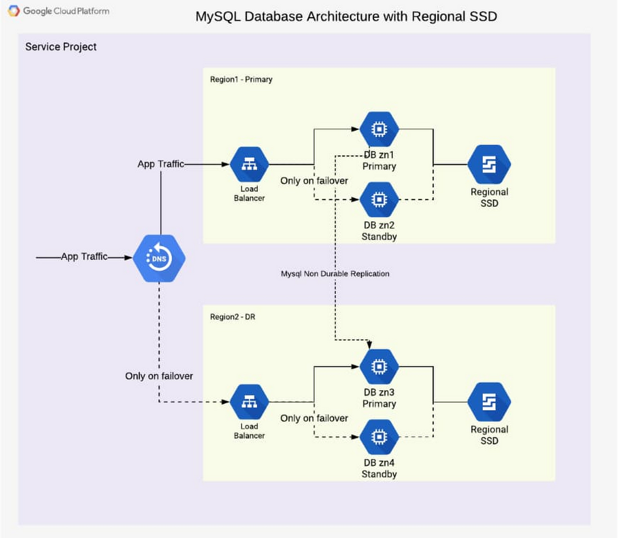
In addition to the database instance setup, a regional disk is deployed so that data is written simultaneously in two zones, proving fail-safe in the event of zone failure. This is a huge advantage of Google Cloud, allowing you to skip MySQL-level replication within a region. Each write operation to disk is done in two zones synchronously. When the primary instance fails, a standby instance is mounted with regional persistent disk(s), and the database service (MySQL) is then started using the same. This brings the peace of mind of not worrying about replication lag or database state for high availability.
From a disaster recovery process view, the following happens over time during a failure situation:
- Normal steady state database operation
- A failure happens and a region becomes unavailable or the database instance inaccessible
- A decision must be made to fail over or not (in case there is the expectation that the region becomes available soon enough or the instance becomes responsive again)
- DNS is updated manually, therefore it redirects application traffic to a second region
- Fallback to the primary region after it becomes available again is optional, as the second region is a fully built-out deployment
From a high-availability process view, the following happens over time during a failure situation:
- Normal steady state database operation
- Database instance fails or becomes unavailable
- Launch the standby instance
- Mount regional SSD and start database
- Automatic redirection of application traffic to the standby via load balancer
- After the failed or unavailable instance becomes available again, a fallback can take place or not
The database architecture shown demonstrates a highly available architecture supporting disaster recovery. With regional disks and load balancers, it is straightforward to provide a resilient database deployment.
Find out more about load balancers and regional disks. Check out general HA and DR processes and detailed steps in the initial part of the reference guide. Try it out to become familiar with the architecture as well as the two major failover processes.
Two Ways to Deploy SAP HANA System on Google Cloud

7885
Of your peers have already read this article.
4:00 Minutes
The most insightful time you'll spend today!
Many of the world’s leading companies run on SAP—and deploying it on Google Cloud extends the benefits of SAP even further. Migrating your current SAP S/4HANA deployment to Google Cloud—whether it resides on your company’s on-premises servers or another cloud service—provides your organization with a flexible virtualized architecture that lets you scale your environment to match your workloads, so you pay only for the compute and storage capacity you need at any given moment. Google Cloud includes built-in features, such as Compute Engine live migration and automatic restart, that minimize downtime for infrastructure maintenance. And it allows you to integrate your SAP data with multiple data sources and process it using Google Cloud technology such as BigQuery to drive data analytics.
SAP server-side architecture consists of two layers: the SAP HANA database, and the Netweaver application layer. In this blog post, we’ll look at the options and steps for moving the database layer to Google Cloud as a lift and shift or rehost, a straightforward approach that entails moving your current SAP environment unchanged onto Google Cloud.
Deploying an SAP HANA system on Google Cloud
Google Cloud offers SAP-certified virtual machines (VMs) optimized for SAP products, including SAP HANA and SAP HANA Enterprise Cloud, as well as dedicated servers for SAP HANA for environments greater than 12TB. (For a complete list of VM and hardware options, visit the Certified and Supported SAP HANA Hardware Directory.)
Before proceeding with a rehost migration to Google Cloud, your current (source) environment and Google Cloud (target) environments should meet these specifications:
Prerequisites:
- The configuration of the Google Cloud environment (i.e., VM resources, SSD storage capacity) should be identical to that of the source environment. If the underlying hardware is different, however, you must use Option 2 for your migration, detailed below.
- Both environments should be running the same operating system (SUSE or RHEL Linux).
- The HANA version, instance number, and system ID (SID) should be identical.
- Schema names must remain the same.
- Establishing the network connection between the on-premises environment and Google Cloud will be required in this phase to support rehost of the SAP application.you can use Cloud VPN or Dedicated Interconnect. Learn more about Dedicated Interconnect and Cloud VPN.
Note: Depending on your internet connection and bandwidth requirements, we recommend using a Dedicated Interconnect over Cloud VPN for production environments.
We offer a number of automated processes to accelerate your cloud journey. To deploy the SAP HANA system on Google Cloud, you can use the Google Cloud Deployment manager or Terraform and Ansible scripts available on GitHub with configuration file templates to define your installation. For more details, see the Google Cloud SAP HANA Planning Guide.
Note: To deploy SAP HANA on Google Cloud machine types that are certified by SAP for production, please review the Certification for SAP HANA on Google Cloud page.
Moving an SAP HANA Database to Google Cloud
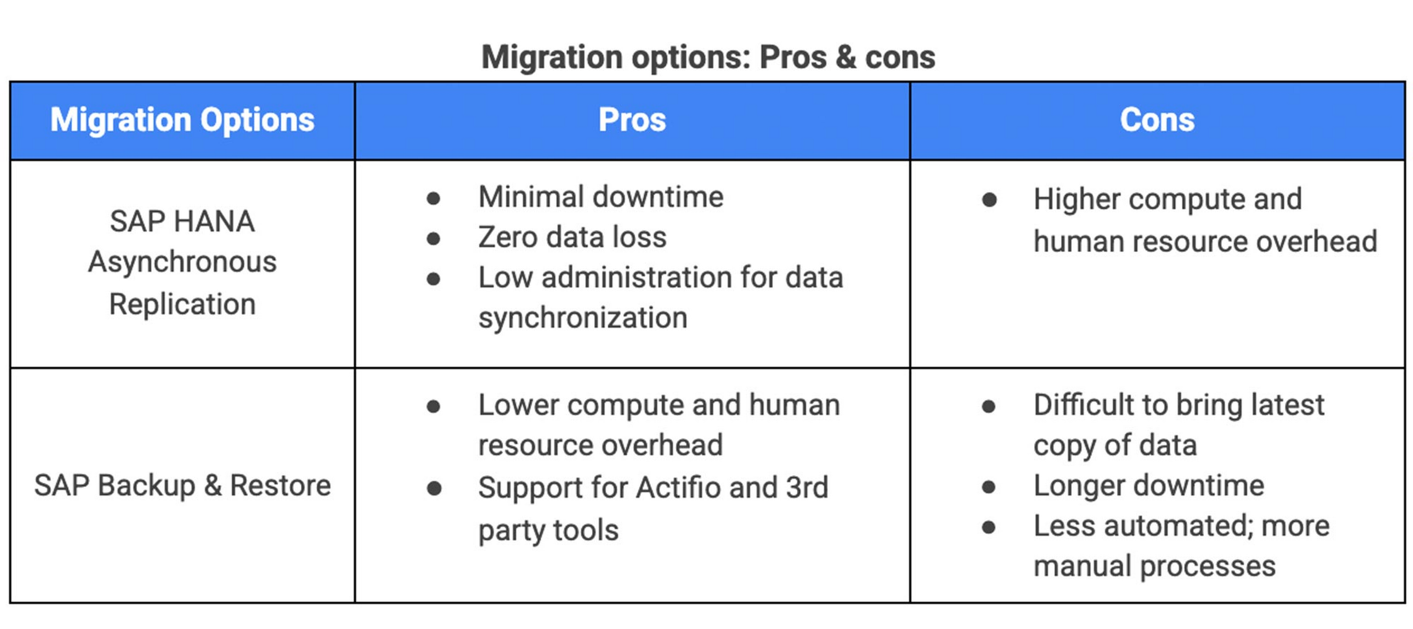
There are two different options you can use to rehost your SAP HANA database to Google Cloud, and each has pros and cons that you should consider when deciding on your approach.
Option 1: Asynchronous replication uses SAP’s built-in replication tool to provide continuous data replication from the source system (also known as the primary system) to the destination or secondary system—in this case residing on Google Cloud. It’s best for mission-critical applications for which minimum downtime is a high priority, and for large databases. In addition, the high level of automation means that the process requires less manual intervention. Here’s where you can learn more on HANA Asynchronous Replication.
Option 2: Backup and restore relies on SAP’s backup utility to create an image of the database that is then transferred to Google Cloud, where it is restored in the new environment. Downtime for this method varies by database size, so large databases may require more downtime via this method vs. asynchronous replication. It also involves more manual tasks. However, it requires fewer resources to perform, making it an attractive option for less urgent use cases. Here’s where you can learn more on SAP HANA database Backup and restore.
How to migrate the SAP HANA database to Google Cloud using Asynchronous Replication
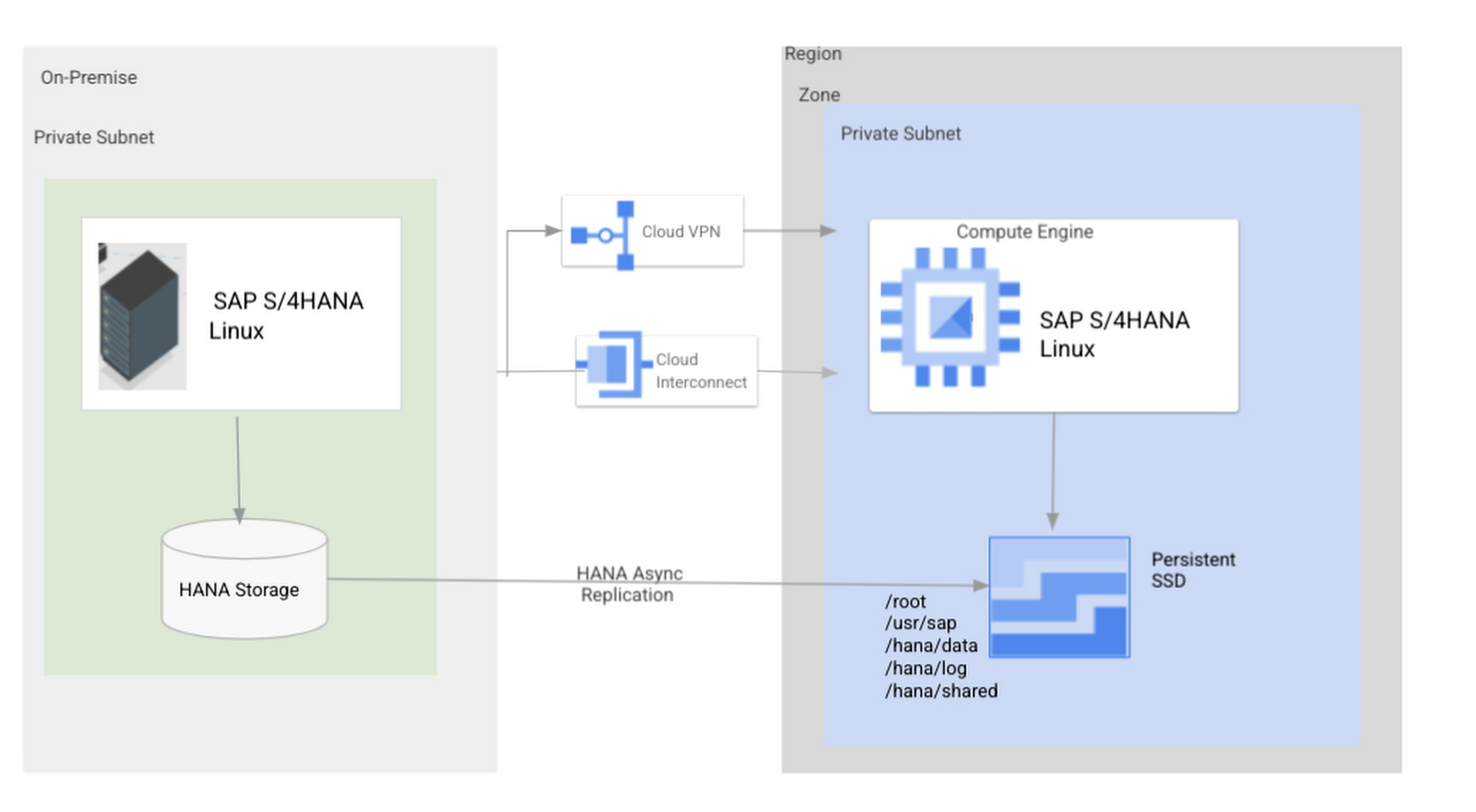
- Create and configure Dedicated Interconnect or Cloud VPN between the current environment and Google Cloud.
- Set up SAP HANA asynchronous replication. You can configure system replication using SAP HANA Cockpit, SAP HANA Studio, or hdbnsutil. See Setting Up SAP HANA System Replication in the SAP HANA Administration Guide.
- Be sure to use the same instance number and HANA SID in the template as the primary instance.
- Configure the Google Cloud instance as the secondary node for using HANA Asynchronous replication.
- Perform data validation once full data replication is completed to the SAP HANA database in Google Cloud. To learn more: HANA System Replication overview.
- Perform an SAP HANA takeover on your standby database. This switches your active system from the current primary system onto the secondary system on Google Cloud. Once the takeover command runs, the system on Google Cloud becomes the new primary system.To learn more: HANA Takeover.
How to migrate the SAP HANA database to Google Cloud using Backup and Restore
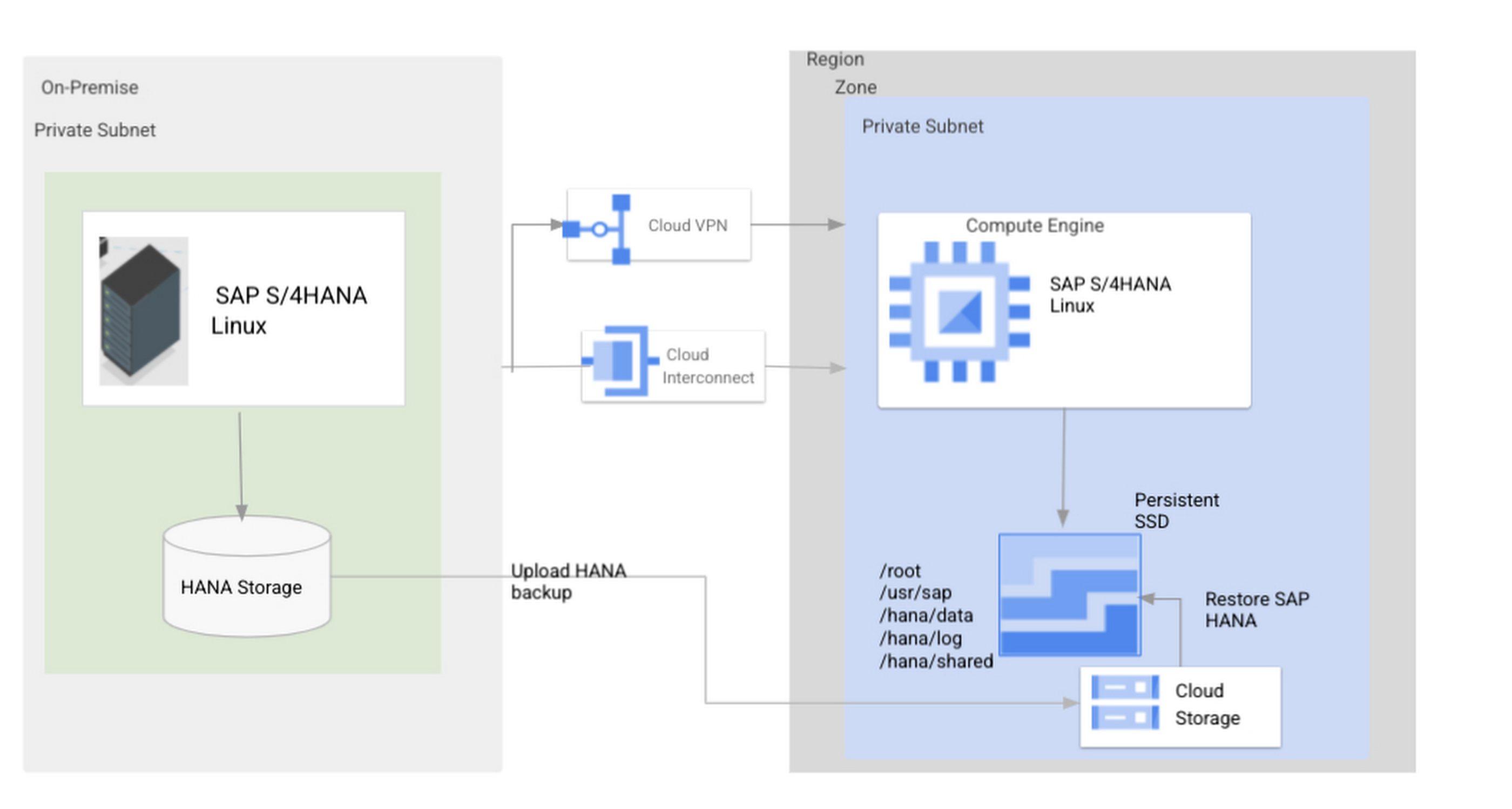
- Create a full backup of your SAP HANA database in your current environment.
- Create a new storage bucket in your Google Cloud environment. Visit Creating Storage Buckets in the Google Cloud Storage documentation.
- Download and install gsutil onto the source environment and run it to upload the HANA backup to the Google Cloud storage bucket. To install gsutil utility on any computer or server, visit Install gsutil in the Google Cloud Storage documentation.
Note: You can run parallel multi thread/multi processing in gsutil to copy large files more quickly. - Recover the HANA database on Google Cloud using SAP’s RECOVER DATABASE statement. See RECOVER DATABASE Statement (Backup and Recovery) in the SAP HANA SQL Reference Guide for SAP HANA Platform.
Note: BackInt agent is an integrated SAP interface tool used for HANA database on Google Cloud.Backint agent for SAP HANA can be used to store and retrieve backups directly from Google Cloud Storage. It is supported and certified by SAP on Google Cloud. To learn more: SAP HANA Backint Agent on Google Cloud.
In summary, we recommend using Asynchronous Replication (Option 1) for mission-critical applications that require the lowest downtime window. For all other applications, we recommend Backup and Restore (Option 2), as this approach requires fewer resources. It’s also a great way to implement the backup and restore functionality on Google Cloud.
A rehost migration is the most straightforward path to getting your SAP on HANA system up and running on Google Cloud. And the sooner you migrate, the sooner you can take advantage of the many benefits Google Cloud brings to your SAP solution. For more information on the different migration options please review: SAP on Google Cloud: Migration strategies.
Learn more about deploying SAP on Google Cloud. Technical resources can be found here.
A Breakdown of Cloud-based Data Ingestion Practices

8819
Of your peers have already read this article.
3:00 Minutes
The most insightful time you'll spend today!
Businesses around the globe are realizing the benefits of replacing legacy data silos with cloud-based enterprise data warehouses, including easier collaboration across business units and access to insights within their data that were previously unseen. However, bringing data from numerous disparate data sources into a single data warehouse requires you to develop pipelines that ingest data from these various sources into your enterprise data warehouse. Historically, this has meant that data engineering teams across the organization procure and implement various tools to do so. But this adds significant complexity to managing and maintaining all these pipelines and makes it much harder to effectively scale these efforts across the organization. Developing enterprise-grade, cloud-native pipelines to bring data into your data warehouse can alleviate many of these challenges. But, if done incorrectly, these pipelines can present new challenges that your teams will have to spend their time and energy addressing.
Developing cloud-based data ingestion pipelines that replicate data from various sources into your cloud data warehouse can be a massive undertaking that requires significant investment of staffing resources. Such a large project can seem overwhelming and it can be difficult to identify where to begin planning such a project. We have defined the following principles for data pipeline planning to begin the process. These principles are intended to help you answer key business questions about your effort and begin to build data pipelines that address your business and technical needs. Each section below details a principle of data pipelines and certain factors your teams should consider as they begin developing their pipelines.
Principle 1: Clarify your objectives
The first principle to consider for pipeline development is clarify your objectives. This can be broadly defined as taking a holistic approach to pipeline development that encompasses requirements from several perspectives: technical teams, regulatory or policy requirements, desired outcomes, business goals, key timelines, available teams and their skill sets, and downstream data users. Clarifying your objectives clearly identifies and defines requirements from each key stakeholder at the beginning of the process and continually checks development against these requirements to ensure the pipelines built will meet these requirements.This is done by first clearly defining the desired end state for each project in a way that addresses a demonstrated business need of downstream data users. Remember that data pipelines are almost always the means to accomplish your end state, rather than the end state itself. An example of an effectively defined end-state is “enabling teams to gain a better understanding of our customers by providing access to our CRM data within our cloud data warehouse” rather than “move data from our CRM to our cloud data warehouse”. This may seem like a merely semantic difference, but framing the problem in terms of business needs helps your teams make technical decisions that will best meet these needs.
After clearly defining the business problem you are trying to solve, you should facilitate requirement gathering from each stakeholder and use these requirements to guide the technical development and implementation of your ingestion pipelines. We recommend gathering stakeholders from each team, including downstream data users, prior to development to gather requirements for the technical implementation of the data pipeline. These will include critical timelines, uptime requirements, data update frequency, data transformation, DevOps needs, and security, policy, or regulatory requirements by which a data pipeline must meet.
Principle 2: Build your team
The second principle to consider for pipeline development is build your team. This means ensuring you have the right people with the right skills available in the right places to develop, deploy, and maintain your data pipelines. After you have gathered your pipeline requirements, you can begin to develop a summary architecture that will be used to build and deploy your data pipelines. This will help you identify the human talent you will need to successfully build, deploy, and manage these data pipelines and identify any potential shortfalls that would require additional support from either third-party partners or new team members.
Not only do you need to ensure you have the right people and skill sets available in aggregate, but these individuals need to be effectively structured to empower them to maximize their abilities. This means developing team structures that are optimized for each team’s responsibilities and their ability to support adjacent teams as needed.
This also means developing processes that prevent blockers to technical development whenever possible, such as ensuring that teams have all of the appropriate permissions they need to move data from the original source to your cloud data warehouse without violating the concept of least privilege. Developers need access to the original data source (depending on your requirements and architecture) in addition to the destination data warehouse. Examples of this are ensuring that developers have access to develop and/or connect to a Salesforce Connected App or read access to specific Search Ads 360 data fields.
Principle 3: Minimize time to value
The third principle to consider for pipeline development is minimize time to value. This means considering the long-term maintenance burden of a data pipeline prior to developing and deploying it in addition to being able to deploy a minimum viable pipeline as quickly as possible. Generally speaking, we recommend the following approach to building data pipelines to minimize their maintenance burden: Write as little code as possible. Functionally, this can be implemented by:
1. Leveraging interface-based data ingestion products whenever possible. These products minimize the amount of code that requires ongoing maintenance and empower users who aren’t software developers to build data pipelines. They can also reduce development time for data pipelines, allowing them to be deployed and updated more quickly.
- Products like Google Data Transfer Service and Fivetran allow for managed data ingestion pipelines by any user to centralize data from SaaS applications, databases, file systems, and other tooling. With little to no code required, these managed services enable you to connect your data warehouse to your sources quickly and easily.
- For workloads managed by ETL developers and data engineers, tools like Google Cloud’s Data Fusion provide an easy-to-use visual interface for designing, managing and monitoring advanced pipelines with complex transformations.
2. Whenever interface-based products or data connectors are insufficient, use pre-existing code templates. Examples of this include templates available for Dataflow that allow users to define variables and run pipelines for common data ingestion use cases, and the Public Datasets pipeline architecture that our Datasets team uses for onboarding.
3. If neither of these options are sufficient, utilize managed services to deploy code for your pipelines. Managed services, such as Dataflow or Dataproc, eliminate the operational overhead of managing pipeline configuration by automatically scaling pipeline instances within predefined parameters.
Principle 4: Increase data trust and transparency
The fourth principle to consider for pipeline development is increase data trust and transparency. For the purposes of this document, we define this as the process of overseeing and managing data pipelines across all tools. Numerous data ingestion pipelines that each leverage different tools or are not developed under a coordinated management plan can result in “tech sprawl”, which significantly increases the management overhead of data ingestion pipelines as the quantity of data pipelines increases. This becomes especially cumbersome if you are subject to service-level agreements, or legal, regulatory, or policy requirements for overseeing data pipelines. Preventing tech sprawl is, by far, the best strategy for dealing with it by developing streamlined pipeline management processes that automate reporting. Although this can theoretically be achieved by building all of your data pipelines using a single cloud-based product, we do not recommend doing so because it prevents you from taking advantage of features and cost optimizations that come with choosing the best product for your use case.
A monitoring service such as Google Cloud Monitoring Service or Splunk that automates metrics, events, and metadata collection from various products, including those hosted in on-premise and hybrid computing environments, can help you centralize reporting and monitoring of your data pipelines. A metadata management tool such as Google Cloud’s Data Catalog or Informatica’s Enterprise Data Catalog can help you better communicate the nuances of your data so users better understand which data resources are best fit for a given use case. This significantly reduces your pipeline’s governance burden by eliminating manual reporting processes that often result in inaccuracies or lagging updates.
Principle 5: Manage costs
The fifth principle to consider for pipeline development is manage costs. This encompasses both the cost of cloud resources and the staffing costs necessary to design, develop, deploy, and maintain your cloud resources. We believe that your goal should not necessarily be to minimize cost, but rather maximizing the value of your investment. This means maximizing the impact of every dollar spent by minimizing waste in cloud resource utilization and human time. There are several factors to consider when it comes to managing costs:
- Use the right tool for the job – Different data ingestion pipelines will have different requirements for latency, uptime, transformations, etc. Similarly, different data pipeline tools have different strengths and weaknesses. Choosing the right tool for each data pipeline can help your pipelines operate significantly more efficiently. This can reduce your overall cost, free up staffing time to focus on the most impactful projects, and make your pipelines much more efficient.
- Standardize resource labeling – Implement and utilize a consistent labeling schema across all tools and platforms to have the most comprehensive view of your organization’s spending. One example is requiring all resources to be labeled by the cost center or team at time of creation. Consistent labeling allows you to monitor your spend across different teams and calculate the overall value of your cloud spending.
- Implement cost controls – If available, leverage cost controls to prevent errors that result in unexpectedly large bills.
- Capture cloud spend – Capture your spend on all cloud resource utilization for internal analysis using a cloud data warehouse and a data visualization tool. Without it, you won’t understand the context of changes in cloud spend and how they correlate with changes in business.
- Make cost management everyone’s job – Managing costs should be part of the responsibilities of everyone who can create or utilize cloud resources. To do this well, we recommend making cloud spend reporting more transparent internally and/or implementing chargebacks to internal cost centers based on utilization.
Long-term, the increased granularity in cost reporting available within Google Cloud can help you better measure your key performance indicators. You can shift from cost-based reporting (i.e. – “We spent $X on BigQuery storage last month”) to value-based reporting (i.e. – “It costs $X to serve customers who bring in $Y revenue”).
To learn more about managing costs, check out Google Cloud’s “Understanding the principles of cost optimization” white paper.
Principle 6: Leverage continually improving services
The sixth principle is leverage continually improving services. Cloud services are consistently improving their performance and stability, even if some of these improvements are not obvious to users. These improvements can help your pipelines run faster, cheaper, and more consistently over time. You can take advantage of the benefits of these improvements by:
- Automating both your pipelines and pipeline management: Not only should data pipelines be automated, but almost all aspects of managing your pipelines can also be automated. This includes pipeline/data lineage tracking, monitoring, cost management, scheduling, access management and more. This helps reduce long-term operational costs of each data pipeline that can significantly alter your value proposition and prevent any manual configurations from negating the benefits of later product improvements.
- Minimizing pipeline complexity whenever possible: While ingestion pipelines are relatively easy to develop using UI-based or managed services, they also require continued maintenance as long as they are in use. The most easily maintained data ingestion pipelines are typically the ones that minimize complexity and leverage automatic optimization capabilities. Any transformation in a data ingestion pipeline is a manual optimization of the pipeline that may struggle to adapt or scale as the underlying services improve. You can minimize the need for such transformations by building ELT (extract, load, transform) pipelines rather than ETL (extract, transform, load) pipelines. This pushes transformations down to the data warehouse that is use a specifically optimized query engine to transform your data rather than manually configured pipelines.
Next steps
If you’re looking for more information about developing your cloud-based data platform, check out our Build a modern, unified analytics data platform whitepaper. You can also visit our data integration site to learn more and find ways to get started with your data integration journey.
Once you’re ready to begin building your data ingestion pipelines, learn more about how Cloud Data Fusion and Fivetran can help you make sure your pipelines address these principles.
How to Pick a Database that is Suitable for Your Application

7028
Of your peers have already read this article.
2:30 Minutes
The most insightful time you'll spend today!
Picking the right database for your application is not easy. The choice depends heavily on your use case—transactional processing, analytical processing, in-memory database, and so on—but it also depends on other factors. This post covers the different database options available within Google Cloud across relational (SQL) and non-relational (NoSQL) databases and explains which use cases are best suited for each database option.

Relational databases
In relational databases information is stored in tables, rows and columns, which typically works best for structured data. As a result they are used for applications in which the structure of the data does not change often. SQL (Structured Query Language) is used when interacting with most relational databases. They offer ACID consistency mode for the data, which means:
- Atomic: All operations in a transaction succeed or the operation is rolled back.
- Consistent: On the completion of a transaction, the database is structurally sound.
- Isolated: Transactions do not contend with one another. Contentious access to data is moderated by the database so that transactions appear to run sequentially.
- Durable: The results of applying a transaction are permanent, even in the presence of failures.
Because of these properties, relational databases are used in applications that require high accuracy and for transactional queries such as financial and retail transactions. For example: In banking when a customer makes a funds transfer request, you want to make sure the transaction is possible and it actually happens on the most up-to-date account balance, in this case an error or resubmit request is likely fine.
There are three relational database options in Google Cloud: Cloud SQL, Cloud Spanner, and Bare Metal Solution.
Cloud SQL: Provides managed MySQL, PostgreSQL and SQL Server databases on Google Cloud. It reduces maintenance cost and automates database provisioning, storage capacity management, back ups, and out-of-the-box high availability and disaster recovery/failover. For these reasons it is best for general-purpose web frameworks, CRM, ERP, SaaS and e-commerce applications.
Cloud Spanner: Cloud Spanner is an enterprise-grade, globally-distributed, and strongly-consistent database that offers up to 99.999% availability, built specifically to combine the benefits of relational database structure with non-relational horizontal scale. It is a unique database that combines ACID transactions, SQL queries, and relational structure with the scalability that you typically associate with non-relational or NoSQL databases. As a result, Spanner is best used for applications such as gaming, payment solutions, global financial ledgers, retail banking and inventory management that require ability to scale limitlessly with strong-consistency and high-availability.
Bare Metal Solution: Provides hardware to run specialized workloads with low latency on Google Cloud. This is specifically useful if there is an Oracle database that you want to lift and shift into Google Cloud. This enables data center retirements and paves a path to modernize legacy applications.
Non-relational databases
Non-relational databases (or NoSQL databases) store compex, unstructured data in a non-tabular form such as documents. Non-relational databases are often used when large quantities of complex and diverse data need to be organized. Unlike relational databases, they perform faster because a query doesn’t have to access several tables to deliver an answer, making them ideal for storing data that may change frequently or for applications that handle many different kinds of data.
For example, an apparel store might have a database in which shirts have their own document containing all of their information, including size, brand, and color with room for adding more parameters later such as sleeve size, collars, and so on.
Qualities that make NoSQL databases fast:
- Eventual consistency: stores usually exhibit consistency at some later point (e.g., lazily at read time)
- Horizontal scaling, usually using hashed distributions
- Typically, they are optimized for a specific workload pattern (i.e., key-value, graph, wide-column)
- Typically, they don’t support cross shard transactions or flexible isolation modes.
Because of these properties, non-relational databases are used in applications that require large scale, reliability, availability, and frequent data changes.They can easily scale horizontally by adding more servers, unlike some relational databases, which scale vertically by increasing the machine size as the data grows. Although, some relations databases such as Cloud Spanner support scale-out and strict consistency.
Non-relational databases can store a variety of unstructured data such as documents, key-value, graphs, wide columns, and more. Here are your non-relational database options in Google Cloud:
- Document databases: Store information as documents (in formats such as JSON and XML). For example: Firestore
- Key-value stores: Group associated data in collections with records that are identified with unique keys for easy retrieval. Key-value stores have just enough structure to mirror the value of relational databases while still preserving the benefits of NoSQL. For example: Datastore, Bigtable, Memorystore
- In-memory database: Purpose-built database that relies primarily on memory for data storage. These are designed to attain minimal response time by eliminating the need to access disks. They are ideal for applications that require microsecond response times and can have large spikes in traffic. For example: Memorystore
- Wide-column databases: Use the tabular format but allow a wide variance in how data is named and formatted in each row, even in the same table. They have some basic structure while preserving a lot of flexibility. For example: Bigtable
- Graph databases: Use graph structures to define the relationships between stored data points; useful for identifying patterns in unstructured and semi-structured information. For example: JanusGraph
There are three non-relational databases in Google Cloud:
- Firestore: Is a serverless document database which scales on demand and acts as a backend-as-a-service. It is DBaaS that increases the speed of building applications. It is perfect for all general purpose uses cases such as ecommerce, gaming, IoT and real time dashboards. With Firestore users can interact with and collaborate on live and offline data making it great for real-time application and mobile apps.
- Cloud Bigtable: Cloud Bigtable is a sparsely populated table that can scale to billions of rows and thousands of columns, enabling you to store terabytes or even petabytes of data. It is ideal for storing very large amounts of single-keyed data with very low latency. It supports high read and write throughput at sub-millisecond latency, and it is an ideal data source for MapReduce operations. It also supports the open-source HBase API standard to easily integrate with the Apache ecosystem including HBase, Beam, Hadoop and Spark along with Google Cloud ecosystem.
- Memorystore: Memorystore is a fully managed in-memory data store service for Redis and Memcached at Google Cloud. It is best for in-memory and transient data stores and automates the complex tasks of provisioning, replication, failover, and patching so you can spend more time coding. Because it offers extremely low latency and high performance, Memorystore is great for web and mobile, gaming, leaderboard, social, chat, and news feed applications.
Conclusion
Choosing a relational or a non-relational database largely depends on the use case. Broadly, if your application requires ACID transactions and your data structure is not going to change much, select a relational database.
In Google Cloud use Cloud SQL for any general-purpose SQL database and Cloud Spanner for large-scale globally scalable, strongly consistent use cases. In general, if your data structure may change later and if scale and availability is a bigger requirement than consistency then a non-relational database is a preferable choice. Google Cloud offers Firestore, Memorystore, and Cloud Bigtable to support a variety of use cases across the document, key-value, and wide column database spectrum.
For more comparison resources on each database check out the overview. For more hands-on experience with Bigtable, check out our on-demand training here and learn about migrating databases to managed services check out this whitepaper.
https://youtube.com/watch?v=2TZXSnCTd7E%3Fenablejsapi%3D1%26
For more #GCPSketchnote, follow the GitHub repo. For similar cloud content follow me on Twitter @pvergadia and keep an eye out on thecloudgirl.dev.
How Arvind Fashions Ltd leads the fashion industry with powerful data analytics on BigQuery

4117
Of your peers have already read this article.
3:30 Minutes
The most insightful time you'll spend today!
Arvind Ltd has been in the apparel industry for more than 90 years, with its retail powerhouse Arvind Fashions Ltd being the backbone of well-known names in the retail fashion industry in India.
Arvind Fashions Ltd (Arvind) has seen significant growth in its portfolio with new franchises being added every year. The six high conviction brands include Tommy Hilfiger, Calvin Klein, Sephora, Arrow, U.S. Polo Assn. & Flying Machine.
To secure a foundation for future growth, the company has embarked on a digital transformation (DX) journey, focusing on profitability and improving the customer experience. The key objectives for Arvind’s DX is to unlock the value of existing applications, gain new insights, and build a solid workflow with resilient systems.
Getting Google Cloud to address the challenges around insights & analytics was a natural step forward, since Arvind had already formed a relationship with Google Cloud, starting with its productivity and collaboration tools during the pandemic.
Key Challenges
Arvind’s enterprise applications estate is a mix of SAP, Oracle POS, logistics management systems and other applications. Having so many different applications made it a challenge for the company to bring all of this data together to drive retail insights and at the same time maintain the freshness of its products.
As a case in point, the existing sales reporting and inventory reconciliation process had been enabled by a mix of automated and semi-automated desktop applications. There were challenges to scale the infrastructure in order to process large amounts of data at a low latency.
The synchronization of master data across functions was critical to build the data platform that provides consistent insights to multiple stakeholders across the organization.
Solution Approach – Modern Data Platform
There are several ways to solve the challenges above and do more by building a modern data analytics platform. For example, using a data lake based approach that builds use case by use case, hybrid data estates and so on. Regardless of the approach, it is important to define the solution based on certain principles.
In Arvind’s scenario, the key business principles considered are that data platforms should support Variety, Variability, Velocity and Volume. Each of these 4 V’s are critical business pivots to successful fashion retailing. Variety in SKU’s to deal with myriad fashion trends every season, Variability in shopping footfalls due to different festivities, weekends and special occasions, Velocity to be agile and responsive to customer needs, and Volumes of data that bring richer insights.
This is where Google BigQuery enabled data platform comes in, as it is able to meet the needs above.
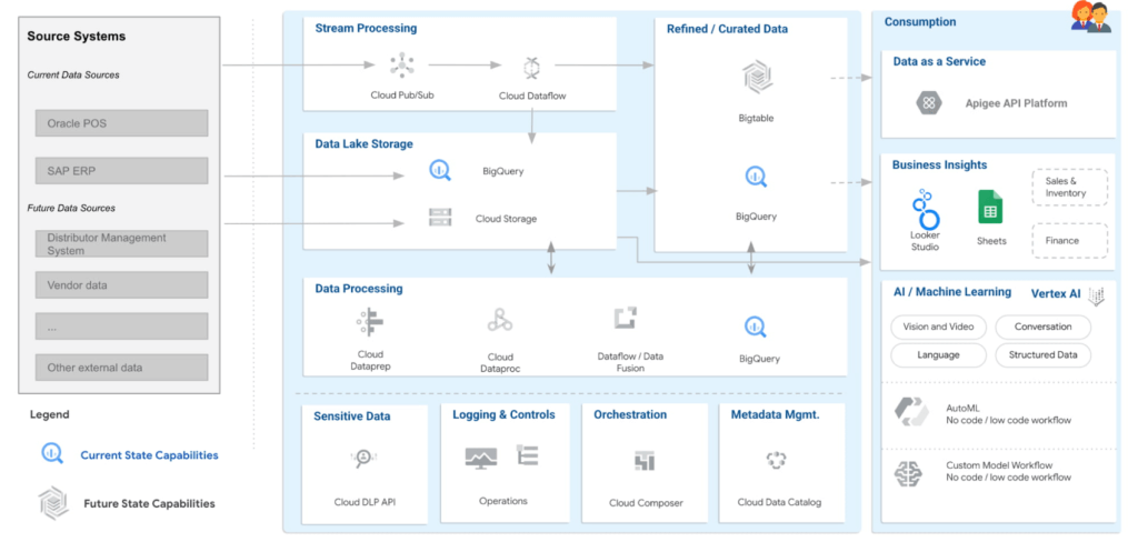
Solution Architecture – Current Capabilities & Future Vision
BigQuery is the mothership of the data and analytics platform on Google Cloud. Its serverless construct ensures that data engineering teams focus only on insights & analytics. Storage and compute is decoupled and can be independently scaled. BigQuery has been leveraged to service both the raw as well as the curated data zones.
With BigQuery procedures, it is possible to process the data natively within the data warehouse itself. Procedures have been leveraged to process the data in a low latency manner with the familiar SQL.
But then what happens to advanced analytics and insights? With simplicity being our key guiding principle, BigQuery machine learning ensures that data analysts can create, train and deploy analytics models even with complex requirements. It can also consume data from Looker Studio, which is seamlessly integrated with BigQuery.
Here are the key principles and highlights of the data platform that have been achieved:
- Simple, yet exhaustive – We needed a solution with vast technical capabilities such as data lake & data warehouse, data processing, data consumption, analytics amongst others. And at the same time it needed to be simple to implement and run ongoing operations.
- Agility – High quality analytics use cases typically require a significant amount of time, effort and skill set. While building a simple solution we ensured that the selection of technology services ensured agility in the long term.
- Security – An organization can be truly successful if the insights and analytics operations are democratized. But while data is made available to a wider community, we need to ensure data governance and security.
- Ease of operations – Data engineering teams spend a lot of time doing infrastructure setting and management operations. With BigQuery, teams can put in more effort on building the data pipelines and models to feed into analytics instead of worrying about the infrastructure operations.
- Costs – Decoupling storage and compute allows for flexible pricing. A pay-as-you-go model is the ideal solution to managing costs.
Business Impact
The ingestion frequency of the store level inventory (~800 stores) has now been changed to daily. With the additional data volumes and processing the scaling on BigQuery has been seamless. There are new processes and dashboards to address the reconciliation and root cause analysis. Operational efficiencies have improved leading to better productivity and turn around time of critical processes.
The discrepancies in various reconciliation activities have drastically reduced by an order of magnitude of 300X due to the capabilities offered by the data platform. Not only is it possible to identify discrepancies but the data platform has also enabled in identifying the root causes for the same as well.
Arvind Fashions Ltd have also been able to enhance some of the existing business processes and systems with insight from the data platform.
It’s going to be an exciting journey for Arvind Fashions Ltd and Google Cloud. There are several initiatives ready for kick off such as getting more apps on the edge devices, warehouse analytics, advanced customer data platforms, predicting the lifecycle of designs, style codes and other exciting initiatives.
Experts’ Guideline for Personalizing Platforms with the Right Recommendation System on Google Cloud

5005
Of your peers have already read this article.
5:00 Minutes
The most insightful time you'll spend today!
Over the past two decades, consumers have become accustomed to receiving personalized recommendations in all facets of their online life. Whether that be recommended products while shopping on Amazon, a curated list of apps in the Google Play store, or relevant videos to watch next on YouTube. In fact, in a Verge article “How YouTube perfected the feed: Google Brain gave YouTube new life,” the Google Brain team reveals how their recommendation engine has impacted the platform with “more than 70 percent of the time people spend watching videos on the site being driven by YouTube’s algorithmic recommendations” thereby increasing time spent on the platform by 20X in three years.
It’s become clear that personalized recommendations are no longer a differentiator for an organization but rather something consumers have come to expect in their day-to-day experiences online. So what should you do if you are behind the curve and want to get started or simply want to improve upon what you already have? While there are all sorts of techniques, from content-based systems to deep learning methods, our goal in this recommender-focused blog series is to demystify three available approaches to building recommendation systems on Google Cloud: Matrix Factorization in BigQuery Machine Learning (BQML), Recommendations AI, and deep retrieval techniques available via the Two-Tower built-in algorithm.
One of these approaches can be used to meet you where you are in your personalization journey, no matter if you are just starting or if you are well into it. This first blog post will introduce our three approaches and when to use them.
What is Matrix Factorization and how does it work?
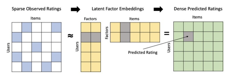
Collaborative filtering is a foundational model for building a recommendation system as the input dataset is simple and the embeddings are learned for you. How does Matrix factorization fit into the mix you might be wondering? Matrix factorization is simply the model that applies collaborative filtering. BQML enables users to create and execute a matrix factorization model by using standard SQL directly in the data warehouse.
Collaborative filtering begins by creating an interaction matrix. The interaction matrix represents users as a row and items as columns in your dataset. This interaction matrix often is sparse in nature as not all users will have interacted with many items in your catalog. This is where embeddings come into play. Generating embeddings for users and items not only allows you to collapse many sparse features into a lower dimensional space but they also allow you to derive a similarity measure so that similar users/items fall nearby in the embedding space. These similarity measures are key as collaborative filtering uses similarities between users and items to make the end recommendations. The underlying assumption being that similar users will like similar items whether that be movies or handbags.
What’s required to get started?
To train a matrix factorization model you need a table that includes three input columns: user(s), item(s), and an implicit or explicit feedback variable (e.g., ratings is an example of explicit feedback). With the base input dataset in place, you can then easily run your model in BigQuery after specifying several hyperparameters in your CREATE MODEL SQL statement. Hyperparameters are available to specify the number of embeddings, the feedback type, the amount of L2 regularization applied and so on.
Why use this approach and who is it a good fit for?
As mentioned earlier, Matrix Factorization in BQML is a great way for those new to recommendation systems to get started. Matrix factorization has many benefits:
- Little ML Expertise: Leveraging SQL to build the model lowers the level of ML expertise needed
- Few Input Features: Data inputs are straightforward, requiring a simple interaction matrix
- Additional Insight: Collaborative filtering is adept at discovering new interests or products for users
While Matrix Factorization is a great tool for deriving recommendations it does come with additional considerations and potential drawbacks depending upon the use case.
- Not Amenable to Large Feature Sets: The input table can only contain two feature columns (e.g., user(s), item(s)). If there is a need to include additional features such as contextual signals, Matrix factorization may not be the right method for you.
- New Items: If an item is not available in the training data, the system can’t create an embedding for it and will have difficulty recommending similar items. While there are some workarounds available to address this cold-start issue, if your item catalog often includes new items, Matrix factorization may not be a good fit.
- Input Data Limitations: While the input matrix is expected to be sparse, training examples without feedback can cause problems. Filtering for items and users that have at least a handful of feedback (e.g., ratings) examples can improve the model. More information on limitations can be found here.
In summary, for users with a simplified dataset looking to iterate quickly and develop a baseline recommendation system, Matrix Factorization is a great approach to begin your personalization AI journey.
What is Recommendations AI and how does it work?
Recommendations AI is a fully managed service which helps organizations deploy scalable recommendation systems that use state-of-the-art deep learning techniques, including cutting-edge architectures such as two-tower encoders, to serve personalized and contextually relevant recommendations throughout the customer journey.
Deep learning models are able to improve the context and relevance of recommendations in part because they can easily address the previously mentioned limitations of Matrix Factorization. They incorporate a wide set of user and item features, and by definition they emphasize learning successive layers of increasingly meaningful representations from these features. This flexibility and expressivity allows them to capture complex relationships like short-lived fashion trends and niche user behaviors. However, this increased relevance comes at a cost, as deep learning recommenders can be difficult to train and expensive to serve at scale.
Recommendations AI helps organizations take advantage of serving these deep learning models and handles the MLOps required to serve these models globally with low latency. Models are automatically retrained daily and tuned quarterly to capture changes in customer behavior, product assortment, pricing, and promotions. Newly trained models follow a resilient CI/CD routine which validates they are fit to serve and promotes them to production without service interruption. The models achieve low serving latency by using a scalable approximate nearest neighbors (ANN) service for efficient item retrieval at inference time. And, to maintain consistency between online and offline tasks, a scalable feature store is used, preventing common production challenges such as data leakage and training-serving skew.
What’s required to get started?
To get started with Recommendations AI we first need to ingest product and user data into the API:
- Import product catalog: For large product catalog updates, ingest catalog items in bulk using the catalogItems.import method. Frequent catalog updates can be schedule with Google Merchant Center or BigQuery
- Record user events: User events track actions such as clicking on a product, adding items to cart, or even purchasing an item. These events need to be ingested in real time to reflect the latest user behavior and then joined to items imported in the product catalog
- Import historical user events: The models need sufficient training data before they can provide accurate predictions. The recommended user event data requirements are different across model types (learn more here)
Once the data requirements are met, we are able to create one or multiple models to serve recommendations:
- Determine your recommendation types and placements: The location of the recommendation panel and the objective for that panel impact model training and tuning. Review the available recommendations types, optimization objectives, and other model tuning options to determine the best options for your business objectives.
- Create model(s): Initial model training and tuning can take 2-5 days depending on the number of user events and size of the product catalog
- Create serving configurations and preview recommendations: After the model is activated, create serving configurations and preview the recommendations to ensure your setup is functioning as expected before serving to production traffic
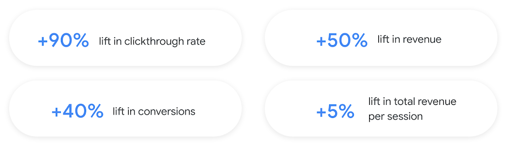
Once models are ready to serve, consider setting up A/B experiments to understand how newly trained models impact your customer experience before serving them to 100% of your traffic. In the Recommendations AI console, see the Monitoring & Analytics page for summary and placement-specific metrics (e.g., recommender-engaged revenue, click-through-rate, conversion rate, and more).
Why use this approach and who is it a good fit for?
Recommendations AI is a great way to engage customers and grow your online presence through personalization. It’s used by teams who lack technical experience with production recommendation systems, as well as customers who have this technical depth but want to allocate their team’s effort towards other priorities and challenges. No matter your team’s technical experience or bandwidth, you can expect several benefits with Recommendations AI:
- Fully managed service: no need to preprocess data, train or hypertune machine learning models, load balance or manually provision you infrastructure – this is all taken care of for you. The recommendation API also provides a user-friendly console to monitor performance over time.
- State-of-the-art AI: take advantage of the same modeling techniques used to serve recommendations across Google Ads, Google Search, and YouTube. These models excel in scenarios with long-tail products and cold-starts users and items
- Deliver at any touchpoint: serve high-quality recommendations to both first-time users and loyal customers anywhere in their journey via web, mobile, email, and more
- Deliver globally: serve recommendations in any language anywhere in the world at low-latency with a fully automated global serving infrastructure
- Your data, your models: Your data and models are yours. They’ll never be used for any other Google product nor shown to any other Google customer
For users looking to leverage state of the art AI to fuel their recommendation systems but need an existing solution to get up and running more quickly, Recommendations AI is the right solution for you.
What are Two Tower encoders and how do they work?
As a reminder, in recommendation system design, our objective is to surface the most relevant set of items for a given user or set of users. The items are usually referred to as the candidate(s) where we might include information about the items such as the title or description of the item, other metadata about the item like language, number of views, or even clicks on the item over time. User(s) are often represented in the form of a query to a recommendation system where we might provide details about the user such as the location of the user, preferred languages, and what they have searched for in the past.
Let’s start with a common example. Imagine that you are creating a movie recommendation system. The input candidates for such a system would be thousands of movies and the query set can consist of millions of viewers. The goal of the retrieval stage is to select a smaller subset of movies(candidates) for each user and then score and rank order them before presenting the final recommended list to the query/user.
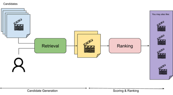
The retrieval stage is able to refine our list of candidates by encoding both the candidate and the query data so they share the same embedding space. A good embedding space will place candidates which are similar to one another closer together and dissimilar items/queries farther apart in the embedding space.
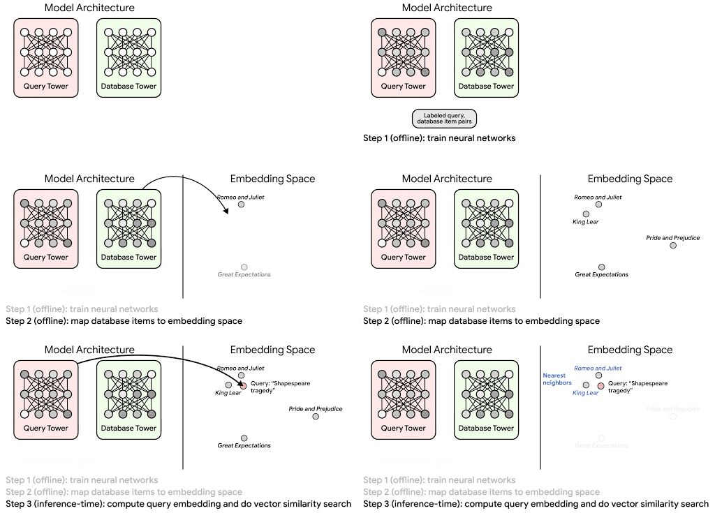
Once we have a database of query and candidate embeddings we can then use an approximate nearest neighbor search method to then generate a list of final “like” candidates, i.e. find a certain number of nearest neighbors for a given query/user and surface final recommendations.
What’s required to get started?
At the most basic level, in order to train a two-tower model you need the following inputs:
- Training Data: Training data is created by combining your query/user data with data about the candidates/items. The data must include matched pairs, cases where both user and item information is available. Data in the training set can include many formats from text, numeric data, or even images.
- Input Schema: The input schema describes the schema of the combined training data along with any specific feature configurations.
Several services within Vertex AI have come available that complement the existing Two-Tower built-in algorithm and can be leveraged in your execution:
- Nearest Neighbor (ANN) Service: Vertex AI Matching Engine and ScANN provide a high-scale and low-latency Approximate Nearest Neighbor (ANN) service so you can more easily identify similar embeddings.
- Hyperparameter Tuning Service: A hyperparameter tuning service such as Vizier can help you identify the optimal hyperparameters such as the number of hidden layers, the size of the hidden layers, and the learning rate in fewer trials.
- Hardware Accelerators: Specialized hardware, such as GPUs or TPUs, can be valuable in your recommendation system to help accelerate experiments and improve the speed of training cycles.
Why use this approach and who is it a good fit for?
The Two-Tower built-in algorithm can be considered the “custom sports car” of recommendation systems and comes with several benefits:
- Greater Control: While Recommendations AI uses the two-tower architecture as one of the available architectures it doesn’t provide granular control or visibility into model training, example generation, and model validation details. In comparison, the Two-Tower built in algorithm provides a more customizable approach as you are training a model directly in a notebook environment.
- More Feature Options: The Two Tower approach can handle additional contextual signals ranging from text to images.
- Cold Start Cases: Leveraging a rich set of features not only enhances performance but also allows the candidate generation to work for new users or new candidates.
While the Two-Tower built in algorithm is an excellent and best-in class solution for deriving recommendations, it does come with additional considerations and potential drawbacks depending upon the use case.
- Technical ML Expertise Required: Two tower encoders are not a “plug and play” solution like the other approaches mentioned above. In order to effectively leverage this approach, appropriate coding and ML expertise is required.
- Speed to Insight: Building out a custom solution via two-tower encoders may require additional time as the solution is not pre-built for the user.
For users looking for greater control, increased flexibility, and have the technical chops to easily work within a managed notebook environment – the two-tower built in algorithm is the right solution for them.
What’s next?
In this article, we explored three common methods for building recommendation systems on Google Cloud Platform. As you can see thus far, there are alot of considerations to take into account before choosing a final approach. In an effort to help you align more quickly we have distilled the decision criteria down to a few simple steps (see below for more details).
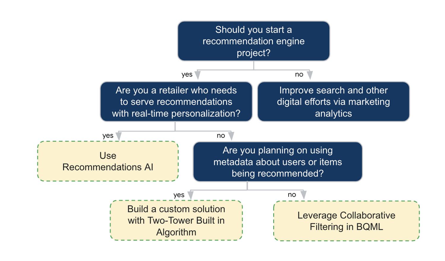
In the next installments of this series, we will dive more deeply into each method, explore how hardware accelerators can play a key role in recommendation system design, and discuss how recommendation systems may be leveraged in key verticals. Stay tuned for future posts in our recommendation systems series. Thank you for reading! Have a question or want to chat? Find authors here – R.E. [Twitter | LinkedIn], Jordan [LinkedIn], and Vaibhav [LinkedIn].
Acknowledgements
Special thanks to Pallav Mehta, Henry Tappen,Abhinav Khushraj, and Nicholas Edelman for helping to review this post.
References
More Relevant Stories for Your Company

Pay-Go Option for MongoDB on Google Cloud Helps Customers Scale as Required
As the volume and velocity of data grows daily, business success depends on the ability to manage it effectively and transform it into actionable insights. Since 2019, Google Cloud and MongoDB have worked together to give businesses the secure, global, and highly performant infrastructure, the sophisticated data intelligence, and the

PaGaLGuY Turns to Google Cloud Platform to Power Leading India Education Network
Founded in 2006, PaGaLGuY started as a forum that enabled students, typically aged between 20 and 30 to discuss and seek advice on academic issues. By 2011, PaGaLGuY had increased its traffic to about 250,000 page views per month. The business is now one of India’s largest education networks and

How Kinguin Notched Up Shopping Experience with Google Recommendations AI
Over 2.14 billion people worldwide are expected to buy online this year, according to Statista. Online retail sales will account for 22% of all purchases by 2023. But in a competitive retail landscape, positive interactions can mean the difference between a sale and an abandoned shopping cart. One of the leading global

Unifying Data and AI: Bringing Unstructured Data Analytics to BigQuery
Over one third of organizations believe that data analytics and machine learning have the most potential to significantly alter the way they run business over the next 3 to 5 years. However, only 26% of organizations are data driven. One of the biggest reasons for this gap is that a
