





Real-time analytics for on-time delivery: Mercado Libre

3051
Of your peers have already read this article.
1:30 Minutes
The most insightful time you'll spend today!
Iteration and innovation fuel the data-driven culture at Mercado Libre. In our first post, we presented our continuous intelligence approach, which leverages BigQuery and Looker to create a data ecosystem on which people can build their own models and processes.
Using this framework, the Shipping Operations team was able to build a new solution that provided near real-time data monitoring and analytics for our transportation network and enabled data analysts to create, embed, and deliver valuable insights.
The challenge
Shipping operations are critical to success in e-commerce, and Mercado Libre’s process is very complex since our organization spans multiple countries, time zones, and warehouses, and includes both internal and external carriers. In addition, the onset of the pandemic drove exponential order growth, which increased pressure on our shipping team to deliver more while still meeting the 48-hour delivery timelines that customers have come to expect.
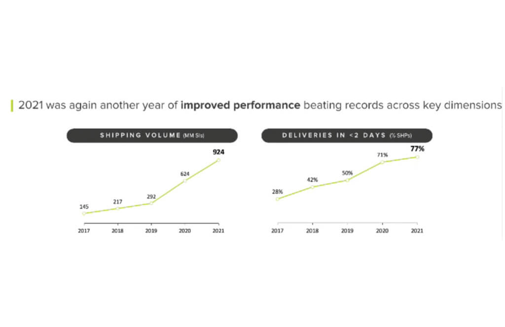
This increased demand led to the expansion of fulfillment centers and cross-docking centers, doubling and tripling the nodes of our network (a.k.a. meli-net) in the leading countries where we operate. We also now have the largest electric vehicle fleet in Latin America and operate domestic flights in Brazil and Mexico.
We previously worked with data coming in from multiple sources, and we used APIs to bring it into different platforms based on the use case. For real-time data consumption and monitoring, we had Kibana, while historical data for business analysis was piped into Teradata. Consequently, the real-time Kibana data and the historical data in Teradata were growing in parallel, without working together. On one hand, we had the operations team using real-time streams of data for monitoring, while on the other, business analysts were building visualizations based on the historical data in our data warehouse.
This approach resulted in a number of problems:
- The operations team lacked visibility and required support to build their visualizations. Specialized BI teams became bottlenecks.
- Maintenance was needed, which led to system downtime.
- Parallel solutions were ungoverned (the ops team used an Elastic database to store and work with attributes and metrics) with unfriendly backups and data bounded for a period of time.
- We couldn’t relate data entities as we do with SQL.
Striking a balance: real-time vs. historical data
We needed to be able to seamlessly navigate between real-time and historical data. To address this need, we decided to migrate the data to BigQuery, knowing we would leverage many use cases at once with Google Cloud.
Once we had our real-time and historical data consolidated within BigQuery, we had the power to make choices about which datasets needed to be made available in near real-time and which didn’t. We evaluated the use of analytics with different time windows tables from the data streams instead of the real-time logs visualization approach. This enabled us to serve near real-time and historical data utilizing the same origin.
We then modeled the data using LookML, Looker’s reusable modeling language based on SQL, and consumed the data through Looker dashboards and Explores. Because Looker queries the database directly, our reporting mirrored the near real-time data stored in BigQuery. Finally, in order to balance near real-time availability with overall consumption costs, we analyzed key use cases on a case-by-case basis to optimize our resource usage.
This solution prevented us from having to maintain two different tools and featured a more scalable architecture. Thanks to the services of GCP and the use of BigQuery, we were able to design a robust data architecture that ensures the availability of data in near real-time.
Streaming data with our own Data Producer Model: from APIs to BigQuery
To make new data streams available, we designed a process which we call the “Data Producer Model” (“Modelo Productor de Datos” or MPD) where functional business teams can serve as data creators in charge of generating data streams and publishing them as related information assets we call “data domains”. Using this process, the new data comes in via JSON format, which is streamed into BigQuery. We then use a 3-tiered transformation process to convert that JSON into a partitioned, columnar structure.
To make these new data sets available in Looker for exploration, we developed a Java utility app to accelerate the development of LookML and make it even more fun for developers to create pipelines.
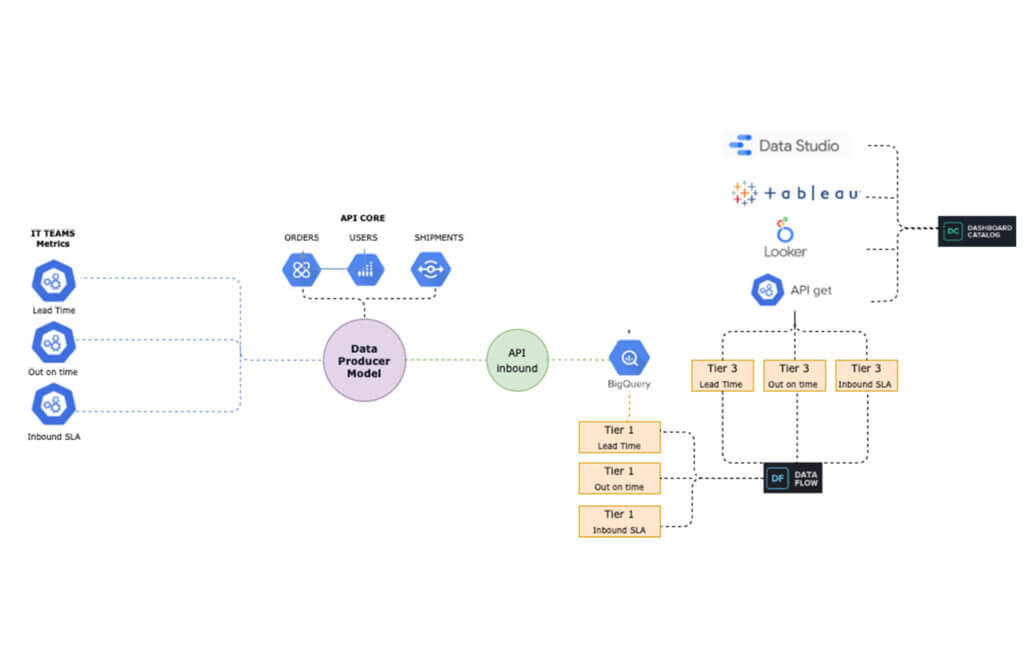
The complete “MPD” solution results in different entities being created in BigQuery with minimal manual intervention. Using this process, we have been able to automate the following:
- The creation of partitioned, columnar tables in BigQuery from JSON samples
- The creation of authorized views in a different GCP BigQuery project (for governance purposes)
- LookML code generation for Looker views
- Job orchestration in a chosen time window
By using this code-based incremental approach with LookML, we were able to incorporate techniques that are traditionally used in DevOps for software development, such as using Lams to validate LookML syntax as a part of the CI process and testing all our definitions and data with Spectacles before they hit production. Applying these principles to our data and business intelligence pipelines has strengthened our continuous intelligence ecosystem. Enabling exploration of that data through Looker and empowering users to easily build their own visualizations has helped us to better engage with stakeholders across the business.
The new data architecture and processes that we have implemented have enabled us to keep up with the growing and ever-changing data from our continuously expanding shipping operations. We have been able to empower a variety of teams to seamlessly develop solutions and manage third party technologies, ensuring that we always know what’s happening – and more critically – enabling us to react in a timely manner when needed.
Outcomes from improving shipping operations:
Today, data is being used to support decision-making in key processes, including:
- Carrier Capacity Optimization
- Outbound Monitoring
- Air Capacity Monitoring
This data-driven approach helps us to better serve you -and everyone- who expects to receive their packages on-time according to our delivery promise. We can proudly say that we have improved both our coverage and speed, delivering 79% of our shipments in less than 48 hours in the first quarter of 2022.
Here is a sneak peek into the data assets that we use to support our day-to-day decision making:
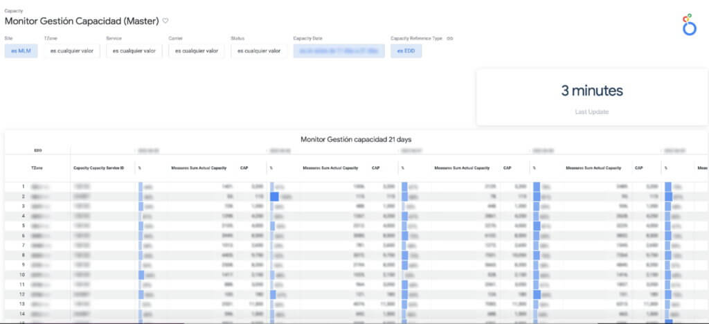
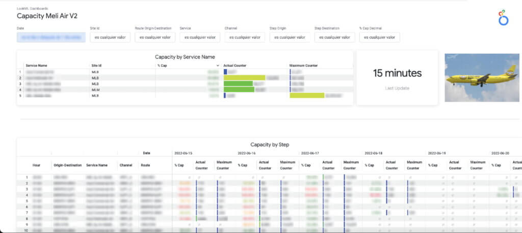
a. Carrier Capacity: Allows us to monitor the percentage of network capacity utilized across every delivery zone and identify where delivery targets are at risk in almost real time.
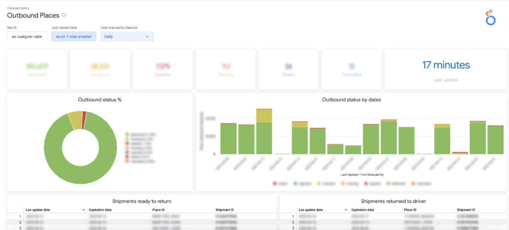
b. Outbound Places Monitoring: Consolidates the number of shipments that are destined for a place (the physical points where a seller picks up a package), enabling us to both identify places with lower delivery efficiency and drill into the status of individual shipments.
c. The Air Capacity Monitoring: Provides capacity usage monitoring for our aircrafts running each of our shipping routes.
Costs into the equation
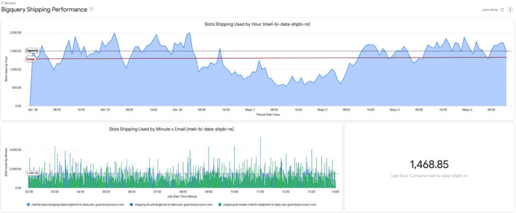
The combination of BigQuery and Looker also showed us something we hadn’t seen before: overall cost and performance of the system. Traditionally, developers maintained focus on metrics like reliability and uptime without factoring in associated costs.
By using BigQuery’s information schema, Looker Blocks, and the export of BigQuery logs, we have been able to closely track data consumption, quickly detect underperforming SQL and errors, and make adjustments to optimize our usage and spend.
Based on that, we know the Looker Shipping Ops dashboards generate a concurrency of more than 150 queries, which we have been able to optimize by taking advantage of BigQuery and Looker caching policies.
The challenges ahead
Using BigQuery and Looker has enabled us to solve numerous data availability and data governance challenges: single point access to near real-time data and to historical information, self-service analytics & exploration for operations and stakeholders across different countries & time zones, horizontal scalability (with no maintenance), and guaranteed reliability and uptime (while accounting for costs), among other benefits.
However, in addition to having the right technology stack and processes in place, we also need to enable every user to make decisions using this governed, trusted data. To continue achieving our business goals, we need to democratize access not just to the data but also to the definitions that give the data meaning. This means incorporating our data definitions with our internal data catalog and serving our LookML definitions to other data visualizations tools like Data Studio, Tableau or even Google Sheets and Slides so that users can work with this data through whatever tools they feel most comfortable using.
If you would like a more indepth look at how we made new data streams available from a process we designed called the “Data Producer Model” (“Modelo Productor de Datos” or MPD) register to attend our webcast on August 31.
While learning and adopting new technologies can be a challenge, we are excited to tackle this next phase, and we expect our users will be too, thanks to a curious and entrepreneurial culture. Are our teams ready to face new changes? Are they able to roll out new processes and designs? We’ll go deep on this in our next post.

Customer Voices: How Firms from Across Industries Leverage Google Cloud
DOWNLOAD CASE STUDY14129
Of your peers have already downloaded this article
1:30 Minutes
The most insightful time you'll spend today!
From powering everyday operations and accelerating application innovation, to providing tools for specific business needs and executing on big ideas, to advancing the security of technology solutions, companies from across industries have leveraged Google Cloud for business benefits.
Companies from across industries have turned to Google Cloud for transforming their business, modernizing their infrastructure, and gleaning intelligence from data. For instance:
- Johnson & Johnson achieved a 41% increase in search results from high-quality job applicants, significantly improving the company’s ability to quickly hire top talent.
- Sony Network Communications now processes 10 billion monthly queries faster, which advances data analysis.
- University College Dublin saw significant 6-figure savings by eliminating legacy hardware, software, and maintenance.
And there are many such examples. Read the collection of case studies to find out how companies from across industries and geographies leveraged Google Cloud for measurable business benefits and for solving complex problems.
Google Cloud Data Heroes Series: Honoring Data Practitioner’s Journey and Learning with GCP

4970
Of your peers have already read this article.
4:00 Minutes
The most insightful time you'll spend today!
Google Cloud Data Heroes is a series where we share stories of the everyday heroes who use our data analytics tools to do amazing things. Like any good superhero tale, we explore our Google Cloud Data Heroes’ origin stories, how they moved from data chaos to a data-driven environment, what projects and challenges they are overcoming now, and how they give back to the community.
For our first issue, we couldn’t be more excited to introduce Google Cloud Data Heroine Lynn Langit. Lynn is a seasoned business woman in Minnesota beginning her eleventh year as the Founder of her own consulting business, Lynn Langit Consulting LLC. Lynn wears many data professional hats including Cloud Architect, Developer, and Educator. If that wasn’t already a handful, she also loves riding her bike at any given season of the year (pictured on the right), which you might imagine gets a bit challenging when you have to invest in bike studded snow tires!

Tell us how you got to be a data practitioner. What was that experience like and how did this journey bring you to GCP?
I worked on the business side of tech for many years. While I enjoyed my work, I found I was intrigued by the nuanced questions practitioners could ask – and the sophisticated decisions they could make – once they unlocked value from their data. This initial intrigue developed into a strong curiosity and I ultimately made the switch from business worker to data practitioner over 15 years ago. This was a huge change in career considering I got my bachelor’s degree in Linguistics and German. And so I started small. I taught myself most everything both at the beginning and even now through online resources, courses, and materials. I began with database and data warehousing, specifically building and tuning many enterprise databases. It wasn’t until Hadoop/NoSQL became available that I pivoted to Big Data…
Back then, I supplemented my self-paced learning with Microsoft technologies, even earning all Microsoft certifications in just one year. When I noticed the industry shifting from on premise to cloud, I shifted my learning from programming to cloud, too. I have been working in the public cloud for over ten years already!
“I started with AWS, but recently I have been doing most everything in GCP. I particularly love implementing data pipelining, data ops, and machine learning.”
How did you supplement your self teachings with Google Cloud data upskilling opportunities like product deep dives and documentation, courses, skills, and certificates?
One of the first Google Cloud data analytics products I fell in love with was BigQuery. BigQuery was my gateway product into a much larger open, intelligent, and unified data platform full of products that combined data analytics, databases, AI/ML, and business intelligence.
I’ve achieved Skills Badges in BigQuery, Data Analysis, and more. I’ve also achieved Google’s Professional Data Engineer Certification, and have been a Google Developer Expert since 2012.
Most recently, I was named one of few Data Analysis Innovator Champions within the Google Cloud Innovators Program, which I’m particularly excited about because I’ve heard it’s a coveted spot for data practitioners and necessitates a Googler nomination to move from the Innovator membership to Champion title!
You’re undoubtedly a data analytics thought leader in the community. When did you know you moved from data student to data master and what data project are you most excited about?
I knew I had graduated, if you will, to the data architect realm once I was able to confidently do data work that matters, even if that work was outside of my usual domains: adTech and finTech..
For example, my work over the past few years has been around human health outcomes, including combatting the COVID-19 pandemic. I do this by supporting scientists and bioinformatic researchers with genomic-scale data pipelines. Did I know anything about genomics before I started? Not at all! I self-studied bioinformatics and recorded my learnings on GitHub. Along the way I adopted my learnings into an open source GCP course on GitHub aimed at researchers who are new to working with GCP. What’s cool about the course is that I begin from the true basics of how to set up a GCP account. Then I gradually work up to mapping out genomic-scale data workflows, pipelines, analyses, batch jobs, and more using BigQuery and a host of other Google Cloud data products.
Now, I’ve received feedback that this repository has made a positive impact on researchers’ ability to process and synthesize enormous amounts of data quickly. Plus, it achieves the greater goal of broadening accessibility to a public cloud like GCP.
In what ways do you think you uniquely bring value back to the data community? Why is it important to you to give back to the data community?
I stay busy always sharing my learnings back to the community. I record Cloud and Big data technical screencasts (demos) on Youtube, I’ve authored 25 data and cloud courses on LinkedIn Learning, and I occasionally write Medium articles on cloud technology and random thoughts I have about everyday life. I’m also the cofounder of Teaching Kids Programming, with a mission to help equip middle and high school teachers with a great programming curriculum on Java.
Begin your own hero’s journey
Ready to embark on your Google Cloud data adventure? Begin your own hero’s journey with GCP’s recommended learning path where you can achieve badges and certifications along the way. Join the Cloud Innovators program today to stay up to date on more data practitioner tips, tricks, and events.
Connect with Google’s data community at our upcoming virtual event “Latest Google Cloud data analytics innovations”. Register and save your spot now to get your data questions answered live by GCP’s top data leaders and watch demos from our latest products and features including BigQuery, Dataproc, Dataplex, Dataflow, and more. Lynn will take the main stage as an emcee for this event – you won’t want to miss!
Finally, if you think you have a good Data Hero story worth sharing, please let us know! We’d love to feature you in our series as well.
How to Enhance Incremental Pipeline Performance while Ingesting Data into BigQuery

6333
Of your peers have already read this article.
3:00 Minutes
The most insightful time you'll spend today!
When you build a data warehouse, the important question is how to ingest data from the source system to the data warehouse. If the table is small you can fully reload a table on a regular basis, however, if the table is large a common technique is to perform incremental table updates. This post demonstrates how you can enhance incremental pipeline performance when you ingest data into BigQuery.
Setting up a standard incremental data ingestion pipeline
We will use the below example to illustrate a common ingestion pipeline that incrementally updates a data warehouse table. Let’s say that you ingest data into BigQuery from a large and frequently updated table in the source system, and you have Staging and Reporting areas (datasets) in BigQuery.

The Reporting area in BigQuery stores the most recent, full data that has been ingested from the source system tables. Usually you create the base table as a full snapshot of the source system table. In our running example, we use BigQuery public data as the source system and create reporting.base_table as shown below. In our example each row is identified by a unique key which consists of two columns: block_hash and log_index.
CREATE TABLE reporting.base_table --156 GB processedPARTITION BY TIMESTAMP_TRUNC(block_timestamp, DAY) ASSELECT log_index, data, topics, block_timestamp, block_hashFROM bigquery-public-data.crypto_ethereum.logsWHERE block_timestamp BETWEEN TIMESTAMP '2020-01-01' AND TIMESTAMP '2020-11-30';
In data warehouses it is common to partition a large base table by a datetime column that has a business meaning. For example, it may be a transaction timestamp, or datetime when some business event happened, etc. The idea is that data analysts who use the data warehouse usually need to analyze only some range of dates and rarely need the full data. In our example, we partition the base table by block_timestamp which comes from the source system.
After ingesting the initial snapshot you need to capture changes that happen in the source system table and update the reporting base table accordingly. This is when the Staging area comes into the picture. The staging table will contain captured data changes that you will merge into the base table. Let’s say that in our source system on a regular basis we have a set of new rows and also some updated records. In our example we mock the staging data as follows: first, we create new data, than we mock the updated records:
CREATE TABLE staging.load_delta AS --5 GB processedSELECT log_index, data, topics, block_timestamp, block_hashFROM bigquery-public-data.crypto_ethereum.logsWHERE block_timestamp BETWEEN TIMESTAMP '2020-12-01' AND TIMESTAMP '2020-12-07';INSERT INTO staging.load_delta --2 GB processedSELECT log_index, CONCAT(data, RAND()), topics, block_timestamp, block_hashFROM bigquery-public-data.crypto_ethereum.logs TABLESAMPLE SYSTEM (5 PERCENT)WHERE block_timestamp BETWEEN TIMESTAMP '2020-10-01' AND TIMESTAMP '2020-11-30';
Next, the pipeline merges the staging data into the base table. It joins two tables by unique key and than updates the changed value or inserts a new row
MERGE INTO reporting.base_table T --161 GB processedUSING staging.load_delta SON T.block_hash = S.block_hashAND T.log_index = S.log_indexWHEN MATCHED THEN UPDATE SETT.data = S.dataWHEN NOT MATCHED THEN INSERT (log_index, data, topics, block_timestamp, block_hash)VALUES (log_index, data, topics, block_timestamp, block_hash);
It is often the case that the staging table contains keys from various partitions but the number of those partitions are relatively small. It holds, for instance, because in the source system the recently added data may get changed due to some initial errors or ongoing processes but older records are rarely updated. However, when the above MERGE gets executed, BigQuery scans all partitions in the base table and processes 161 GB of data. You might add additional join condition on block_timestamp:
MERGE INTO reporting.base_table T --161 GB processedUSING staging.load_delta SON T.block_hash = S.block_hashAND T.log_index = S.log_indexAND T.block_timestamp = S.block_timestampWHEN MATCHED THEN UPDATE SETT.data = S.dataWHEN NOT MATCHED THEN INSERT (log_index, data, topics, block_timestamp, block_hash)VALUES (log_index, data, topics, block_timestamp, block_hash);
But BigQuery would still scan all partitions in the base table because condition T.block_timestamp = S.block_timestamp is a dynamic predicate and BigQuery doesn’t automatically push such predicates down from one table to another in MERGE.
Can you improve the MERGE efficiency by making it scan less data? The answer is Yes.
As described in the MERGE documentation, pruning conditions may be located in a subquery filter, a merge_condition filter, or a search_condition filter. In this post we show how you can leverage the first two. The main idea is to turn a dynamic predicate into a static predicate.
Steps to enhance your ingestion pipeline
The initial step is to compute the range of partitions that will be updated during the MERGE and store it in a variable. As was mentioned above, in data ingestion pipelines, staging tables are usually small so the cost of the computation is relatively low.
DECLARE src_range STRUCT<date_min TIMESTAMP, date_max TIMESTAMP> --115 MB processedDEFAULT(SELECT STRUCT(MIN(block_timestamp) AS date_min,MAX(block_timestamp) AS date_max) FROM staging.load_delta);
Based on your existing ETL/ELT pipeline, you can add the above code as-is to your pipeline or you can compute date_min, data_max as part of some already existing transformation step. Alternatively, date_min, data_max can be computed on the Source System side while capturing the next ingestion data batch.
After computing date_min, date_max you pass those values to the MERGE statement as static predicates. There are several ways to enhance the MERGE and prune partitions in the base table based on precomputed date_min, data_max.
If your initial MERGE statement uses a subquery, you can incorporate a new filter into it:
BEGINDECLARE src_range STRUCT<date_min TIMESTAMP, date_max TIMESTAMP> --115 MB processedDEFAULT(SELECT STRUCT(MIN(block_timestamp) AS date_min,MAX(block_timestamp) AS date_max) FROM staging.load_delta);MERGE INTO reporting.base_table T --41 GB processedUSING (SELECT *FROM staging.load_deltaWHERE block_timestamp BETWEEN src_range.date_min AND src_range.date_max) SON T.block_hash = S.block_hashAND T.log_index = S.log_indexAND T.block_timestamp = S.block_timestampWHEN MATCHED THEN UPDATE SETT.data = S.dataWHEN NOT MATCHED THEN INSERT (log_index, data, topics, block_timestamp, block_hash)VALUES (log_index, data, topics, block_timestamp, block_hash);END;
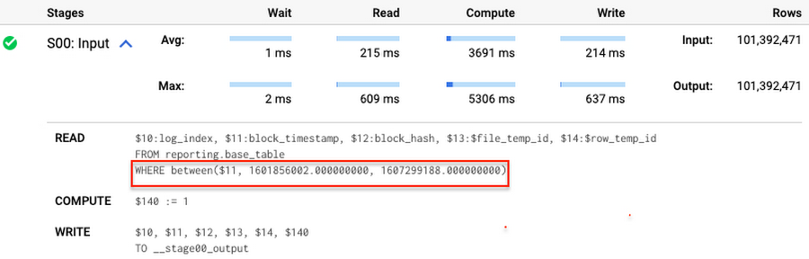
Note that you add the static filter to the staging table and keep T.block_timestamp = S.block_timestamp to convey to BigQuery that it can push that filter to the base table. This MERGE processes 41 GB of data in contrast to the initial 161 GB. You can see in the query plan that BigQuery pushes the partition filter from the staging table to the base table:
This type of optimization, when a pruning condition is pushed from a subquery to a large partitioned or clustered table, is not unique for MERGE. It also works for other types of queries. For instance:
SELECT * -- 41 GB processedFROM reporting.base_table TINNER JOIN staging.load_delta SON T.block_hash = S.block_hashAND T.log_index = S.log_indexAND T.block_timestamp = S.block_timestampWHERE S.block_timestamp BETWEEN TIMESTAMP '2020-10-05' AND TIMESTAMP '2020-12-07'
And you can check the query plan to verify that BigQuery pushed down the partition filter from one table to another.
Moreover, for SELECT statements, BigQuery can automatically infer a filter predicate on a join column and push it down from one table to another if your query meets the following criteria:
- The target table must be clustered or partitioned.
- The result size of the other table, i.e. after applying all filters, must qualify for broadcast join. Namly, the result set must be relatively small, less than ~100MB.
In our running example, reporting.base_table is partitioned by block_timestamp. If you define a selective filter on staging.load_delta and join two tables, you can see an inferred filter on the join key pushed to the target table
SELECT *FROM reporting.base_table TINNER JOIN staging.load_delta SON T.block_timestamp = S.block_timestampWHERE S.block_hash = '0x0c1caa16b34d94843aabfebc0d5a961db358135988f7498a6fdc450ad55f0870'
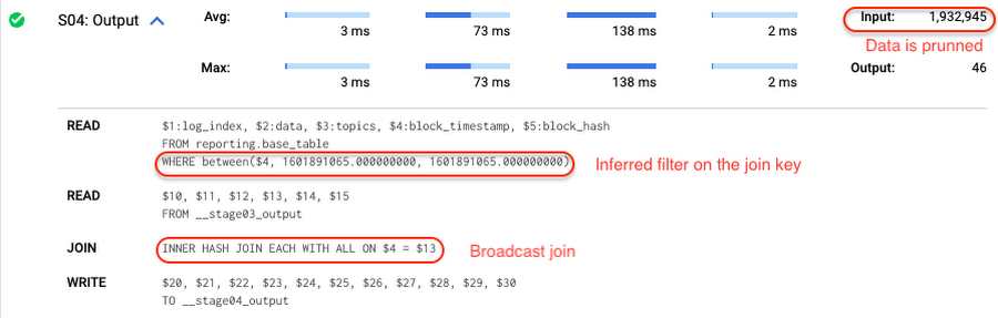
There is no requirement to join tables by partitioning or clustering key to kick off this type of optimization. However, in this case the pruning effect on the target table would be less significant.
But let us get back to the pipeline optimizations. Another way to enhance MERGE is to modify the merge_condition filter by adding static predicate on the base table:
BEGINDECLARE src_range STRUCT<date_min TIMESTAMP, date_max TIMESTAMP> --115 MB processedDEFAULT(SELECT STRUCT(MIN(block_timestamp) AS date_min,MAX(block_timestamp) AS date_max) FROM staging.load_delta);MERGE INTO reporting.base_table T --41 GB processedUSING staging.load_delta SON T.block_hash = S.block_hashAND T.log_index = S.log_indexAND T.block_timestamp BETWEEN src_range.date_min AND src_range.date_maxWHEN MATCHED THEN UPDATE SETT.data = S.dataWHEN NOT MATCHED THEN INSERT (log_index, data, topics, block_timestamp, block_hash)VALUES (log_index, data, topics, block_timestamp, block_hash);END;
To summarize, here are the steps that you can perform to enhance incremental ingestion pipelines in BigQuery. First you compute the range of updated partitions based on the small staging table. Next, you tweak the MERGE statement a bit to let BigQuery know to prune data in the base table.
All the enhanced MERGE statements scanned 41 GB of data, and setting up the src_range variable took 115 MB. Compare it with the initial 161 GB scan. Moreover, given that computing src_range may be incorporated into some existing transformation in your ETL/ELT, it results in a good performance improvement which you can leverage in your pipelines.
In this post we described how to enhance data ingestion pipelines by turning dynamic filter predicates into static predicates and letting BiQuery prune data for us. You can find more tips on BigQuery DML tuning here.
Special thanks to Daniel De Leo, who helped with examples and provided valuable feedback on this content.
Make Meaningful Analysis with Geo Boundary Public Datasets on BigQuery

6353
Of your peers have already read this article.
4:00 Minutes
The most insightful time you'll spend today!
Geospatial data is a critical component for a comprehensive analytics strategy. Whether you are trying to visualize data using geospatial parameters or do deeper analysis or modeling on customer distribution or proximity, most organizations have some type of geospatial data they would like to use – whether it be customer zipcodes, store locations, or shipping addresses. However, converting geographic data into the correct format for analysis and aggregation at different levels can be difficult. In this post, we’ll walk through some examples of how you can leverage the Google Cloud platform alongside Google Cloud Public Datasets to perform robust analytics on geographic data. The full queries can be accessed from this notebook here.
Public US Geo Boundaries dataset
BigQuery hosts a slew of public datasets for you to access and integrate into your analytics. Google pays for the storage of these datasets and provides public access to the data via the bigquery-public-data project. You only pay for queries against the data. Plus, the first 1 TB per month is free! These public datasets are valuable on their own, but when joined against your own data they can unlock new analytics use cases and save the team a lot of time.
Within the Google Cloud Public Datasets Program there are several geographic datasets. Here, we’ll work with the geo_us_boundaries dataset, which contains a set of tables that have the boundaries of different geospatial areas as polygons and coordinates based on the center point (GEOGRAPHY column type in BigQuery), published by the US Census Bureau.
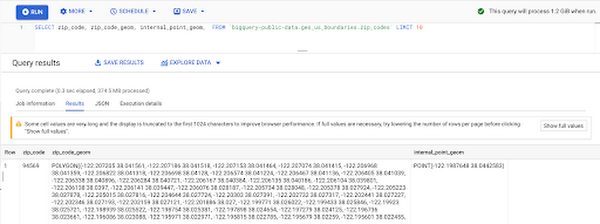
Mapping geospatial points to hierarchical areas
Many times you will find yourself in situations where you have a string representing an address. However, most tools require lat/long coordinates to actually plot points. Using the Google Maps Geocoding API we can convert an address into a lat/long and then store the results in the BigQuery table.
With a lat/long representation of our point, we can join our initial dataset back onto any of the tables here using the ST_WITHIN function. This allows us to check and see if a point is within the specified polygon.
ST_WITHIN(geography_1, geography_2)
This can be helpful for ensuring standard nomenclature; for example, metropolitan areas that might be named differently. The query below maps each customers’ address to a given metropolitan area name.
SELECTcust.id as customer_id,metro.name as metro_nameFROM `looker-private-demo.retail.customers` as cust,`bigquery-public-data.geo_us_boundaries.metropolitan_divisions` as metroWHERE ST_WITHIN(ST_GEOGPOINT(cust.longitude, cust.latitude),metro.metdiv_geom)
It can also be useful for converting to designated market area (DMA), which is often used in creating targeted digital marketing campaigns.
SELECTcust.id as customer_id,dma.dma_nameFROM `looker-private-demo.retail.customers` as cust,`bigquery-public-data.geo_us_boundaries.designated_market_area` as dmaWHERE ST_WITHIN(ST_GEOGPOINT(cust.longitude, cust.latitude),dma.dma_geom)
Or for filling in missing information; for example, some addresses may be missing zip code which results in incorrect calculations when aggregating up to the zipcode level. By joining onto the zip_codes table we can ensure all coordinates are mapped appropriately and aggregate up from there.
SELECTzip.zip_code,count(distinct cust.id) as unique_customersFROM `looker-private-demo.retail.customers` as cust,`bigquery-public-data.geo_us_boundaries.zip_codes` as zipWHERE ST_WITHIN(ST_GEOGPOINT(cust.longitude, cust.latitude),zip.zip_code_geom)GROUP BY 1
Note that the zip code table isn’t a comprehensive list of all US zip codes, they are zip code tabulation areas (ZCTAs). Details about the differences can be found here. Additionally, the zip code table gives us hierarchical information, which allows us to perform more meaningful analytics. One example is leveraging hierarchical drilling in Looker. I can aggregate my total sales up to the country level, and then drill down to state, city and zipcode to identify where sales are highest. You can also use the BigQuery GeoViz tool to visualize geospatial data!
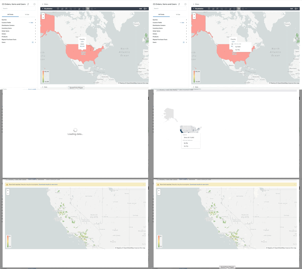
Aside from simply checking if a point is within an area, we can also use ST_DISTANCE to do something like find the closest city using the centerpoint for the metropolitan area table.
SELECTcust.id as customer_id,ARRAY_AGG(metro.name order by ST_DISTANCE(ST_GEOGPOINT(cust.longitude, cust.latitude),metro.internal_point_geom) asc limit 1)[offset(0)] as metro_nameFROM`looker-private-demo.retail.customers` as cust,`bigquery-public-data.geo_us_boundaries.metropolitan_divisions` as metroGROUP BY cust.id
This concept doesn’t just hold true for points, we can also leverage other GIS functions to see if a geospatial area is contained within areas that are listed in the boundaries datasets. If your data comes into BigQuery as a GeoJSON string, we can convert it to a GEOGRAPHY type using the ST_GEOGFROMGEOJSON function. Once our data is in a GEOGRAPHY type we can do things like check to see what urban area the geo is within – using either ST_WITHIN or ST_INTERSECTS to account for partial coverage. Here, I am using the customer’s zip code to find all metropolitan divisions where the zip code polygon and the metropolitan polygon intersect. I am then selecting the metropolitan area that has the most overlap (or the intersection has the largest area) to be the customer’s metro that we use for reporting.
SELECTcust.id as customer_id,ARRAY_AGG(metro.name order by ST_AREA(ST_INTERSECTION(zip.zip_code_geom,metro.metdiv_geom)) desc limit 1)[offset(0)] as metro_nameFROM`looker-private-demo.retail.customers` as custJOIN `bigquery-public-data.geo_us_boundaries.zip_codes` as zip on cust.zip=zip.zip_code,`bigquery-public-data.geo_us_boundaries.metropolitan_divisions` as metroWHERE ST_INTERSECTS(zip.zip_code_geom,metro.metdiv_geom)GROUP BY cust.id
The same ideas can be applied to the other tables in the dataset including the county, urban areas and National Weather Service forecast regions (which can also be useful if you want to join your datasets onto weather data).
Correcting for data discrepancy
One problem that we may run into when working with geospatial data is that different data sources may have different representations of the same information. For example, you might have one system that records state as a two letter abbreviation and another using the full name. Here, we can use the state table to join the different datasets.
SELECTst.state_name,sum(ab.sales+fn.sales) as total_salesFROM `bigquery-public-data.geo_us_boundaries.states` as stLEFT JOIN abbreviated_table as ab on ab.state = st.stateLEFT JOIN fullname_table as fn on fn.state = st.state_nameWHERE COALESCE(ab.state, fn.state) IS NOT NULLGROUP BY 1
Another example might be using the tables as a source of truth for fuzzy matching. If the address is a manually entered field somewhere in your application, there is a good chance that things will be misspelled. Different representations of the same name may prevent tables from joining with each other or lead to duplicate entries when performing aggregations. Here, I use a simple Soundex algorithm to generate a code for each county name, using helper functions from this blog post. We can see that even though some are misspelled they have the same Soundex code.
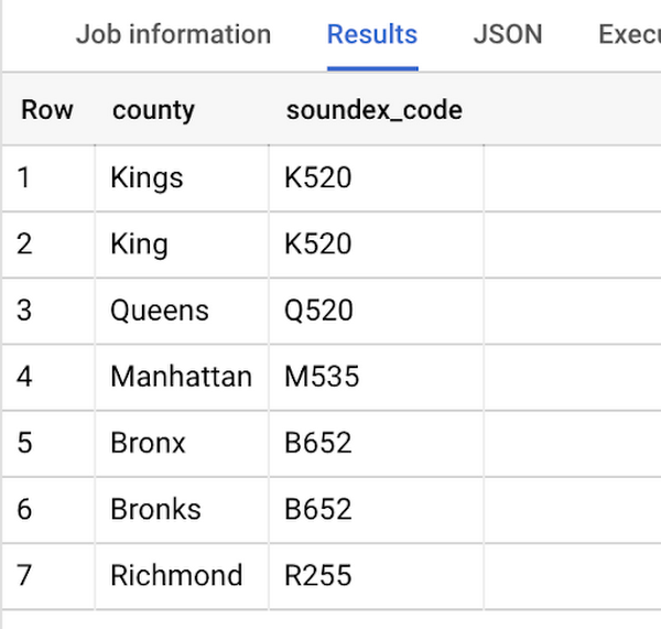
Next, we can join back onto our counties table so we make sure to use the correct spelling of the county name. Then, we can simply aggregate our data for more accurate reporting.
SELECTc.county_name,sum(sales) as total_salesFROMtableJOIN `bigquery-public-data.geo_us_boundaries.counties` as con testing.dq_fm_Soundex(table.county) = testing.dq_fm_Soundex(c.county_name)WHERE c.state_fips_code = cast(36 as string)GROUP BY 1
Note that fuzzy matching definitely isn’t perfect and you might need to try different methods or apply certain filters for it to work best depending on the specifics of your data.
The US Geo Boundary datasets allow you to perform meaningful geographic analysis without needing to worry about extracting, transforming or loading additional datasets into BigQuery. These datasets, along with all the other Google Cloud Public Datasets, will be available in the Analytics Hub. Please sign up for the Analytics Hub preview, which is scheduled to be available in the third quarter of 2021, by going to g.co/cloud/analytics-hub.
Creating and Using Storage Buckets for Your Data Needs

1390
Of your peers have already read this article.
2:30 Minutes
The most insightful time you'll spend today!
So, you want to store objects on the cloud? But you’re really new to Google Cloud or Cloud Storage and would like someone to walk you through the process step by step?
Today is your lucky day!
I will help you understand the big steps involved in setting up and using Cloud Storage. For a walkthrough of all the steps involved that even includes highlighting of things to select so you don’t spend all your time playing “Where’s Waldo” on the page looking for that one button, click try the tutorial!
Creating buckets, storing objects in them, and adjusting permissions may feel challenging at first, but after you’ve walked through these steps, you’ll be able to create and use the Cloud Storage your project needs.
Resource Hierarchy
Projects contain all of the related parts of your application. Inside projects, you may have buckets, the top level containers in Cloud Storage. Files and folders are stored in buckets. You can grant access to a bucket, folder, or file using Identity and Access Management.
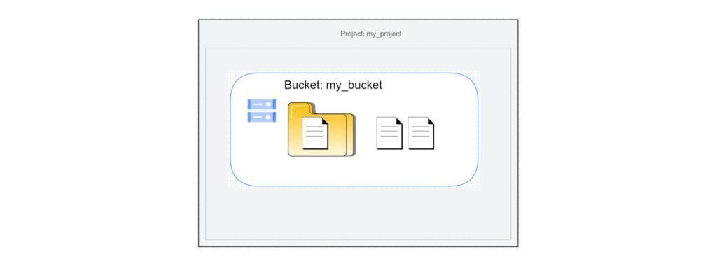
You can do all of that in this interactive tutorial. So let’s get started. I suggest you follow along in the tutorial so you can see the specific keys and screens as I describe them.
Creating a project
Everything in your application will be in a project, even if the only service you are using is storage. Projects need to be associated with a billing account, so if you don’t have one, consider signing up for the Free Trial. You’ll start in the Cloud Console.
Creating a bucket
Once you have a project, you can use storage by navigating to the Cloud Storage page by using either the Navigation menu at the top left of the console or by searching for “Cloud Storage” using the search box at the top of the console.
At the Buckets page of Cloud Storage, you’ll be able to create a bucket. The name of your bucket needs to be globally unique; that is no other bucket in Google Cloud Storage can have the same name. This is because if you or your organization allow your bucket to be accessible on the Internet, it will be at the URL https://storage.googleapis.com/<bucket name>. You can also consider implementing a security feature to prevent data exfiltration, organization restriction headers when you’re finished creating your bucket.. Pick a region close to you for your bucket. In some cases it may make sense to use multi-region or dual-region, but the details are more than I want to get into here. Don’t worry; you can find lots more information on them! Additionally, I won’t go into the details about selecting the appropriate storage class based on access frequency and longevity, but more information can be found here as well our recently introduced Autoclass tiering feature..
Since buckets can be accessed from the Internet, you need to be careful to only make the things you want to be public, public. The default value is to keep your data off of the Internet, so when you create the bucket, there’s an option to “Enforce public access prevention on this bucket” that is already selected. Since we’ll be making items in this bucket public later on, clear the option before confirming the bucket information. Don’t worry; you’ll see how to set that option back later.
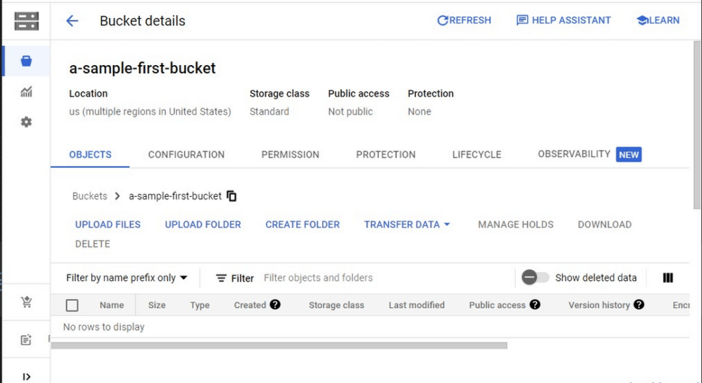
Take a look at the Bucket detail page. There are tabs to see the objects in the bucket, the permissions on the bucket, and much more. There are commands to create folders and to upload files and folders. We’ll do some of this in the next section. You can even find out much more from the Learn option in the upper right.
Adding items to the bucket
Find a file you’d like to upload to this bucket, remembering it will be made public to the Internet later. If you don’t have anything available, there’s a picture of a cat (of course, it’s a cat picture, this is the Internet!) in the interactive tutorial.
Go to the bucket details for your bucket. Using the “Upload files” button, you’ll just upload the file to the bucket by selecting the file from your computer. We won’t get into service classes here, but when you’re ready, there are links in the references.
Of course, if you have a lot of files in a bucket, you probably will want some sort of organization. You can do this by creating folders in your bucket with the “Create Folder” option. Once you’ve done that, you can go to the overflow menu (three vertical dots at the end line with the object information) and select Move. Remember, if you need help finding this, the interactive tutorial will point it out.
Making a bucket public
No surprise, the Bucket details hold lots of information about your bucket. You’ll change the bucket’s permissions in the Permission tab. (I hope that’s not a surprise.) You can then give access to individuals, groups, or all users. For this tutorial, follow the steps to grant access to allUsers. There are a variety of different levels of access you can grant to a user. In this case, just grant the ability to view the object using Storage Object Viewer.
Then go into the Objects tab to find the URL for the object you uploaded. Copy that URL and ensure you can indeed access the object from another tab or incognito window.
Now that you’ve done that, go back to the Permission tab for the bucket and select Prevent Public Access to secure the bucket again.
So, in a nutshell, to make all files in a bucket public, in the Permissions tab:
- Uncheck the option “Remove Public Access Prevention”
- Use Grant Access to give allUsers the Storage Object Viewer role in Cloud Storage.
To make all files in a bucket private, in the Permissions tab select Prevent Public Access.
Cleaning up
There is a charge to keep items in Cloud Storage, so you’ll probably want to delete the object you uploaded by selecting it and pressing Delete. You can delete the bucket in a similar way. The tutorial has details, of course.
While there are lots more details about Cloud Storage, you’ve got the big picture now. Go do something creative and useful with it!
So what now?
If you haven’t walked through the interactive tutorial, give it a try!
More Relevant Stories for Your Company

Bitly’s Big Move: A Story of Massive Data Migration to Google’s Cloud Bigtable
Editor’s note: Bitly, the link & QR Code management platform, migrated 80 billion rows of link data to Cloud Bigtable. Here’s how and why they moved this data from a MySQL database, all in just six days. Our goal at Bitly is simple: Make your life easier with connections. Whether you're sharing




Explore the Innovations and Architecture Powering Spanner and BigQuery
Previously, databases had architectures with tightly coupled storage and compute. This resulted in higher latency, and with faster networks these constraints no longer surface. With Google Cloud's BigQuery and CloudSpanner, the storage and compute architecture have been separated, allowing for better scalability and availability to address businesses' high throughput data

PaGaLGuY Turns to Google Cloud Platform to Power Leading India Education Network
Founded in 2006, PaGaLGuY started as a forum that enabled students, typically aged between 20 and 30 to discuss and seek advice on academic issues. By 2011, PaGaLGuY had increased its traffic to about 250,000 page views per month. The business is now one of India’s largest education networks and

Four Key Takeaways from Google and Quantum Metric’s Back-to-School Retail Benchmark Study
Is it September yet? Hardly! School is barely out for the summer. But according to Google and Quantum Metric research, the back-to-school and off-to-college shopping season – which in the U.S. is second only to the holidays in terms of purchasing volume1 – has already begun. For retailers, that means
