





BigQuery Explainable AI for Demystifying the Inner Workings of ML Models. Now GA!

6558
Of your peers have already read this article.
2:00 Minutes
The most insightful time you'll spend today!
Explainable AI (XAI) helps you understand and interpret how your machine learning models make decisions. We’re excited to announce that BigQuery Explainable AI is now generally available (GA). BigQuery is the data warehouse that supports explainable AI in a most comprehensive way w.r.t both XAI methodology and model types. It does this at BigQuery scale, enabling millions of explanations within seconds with a single SQL query.
Why is Explainable AI so important? To demystify the inner workings of machine learning models, Explainable AI is quickly becoming an essential and growing need for businesses as they continue to invest in AI and ML. With 76% of enterprises now prioritizing artificial intelligence (AI) and machine learning (ML) over other initiatives in 2021 IT budgets, the majority of CEOs (82%) believe that AI-based decisions must be explainable to be trusted according to a PwC survey.
While the focus of this blogpost is on BigQuery Explainable AI, Google Cloud provides a variety of tools and frameworks to help you interpret models outside of BigQuery, such as with Vertex Explainable AI, which includes AutoML Tables, AutoML Vision, and custom-trained models.
So how does Explainable AI in BigQuery work exactly? And how might you use it in practice?
Two types of Explainable AI: global and local explainability
When it comes to Explainable AI, the first thing to note is that there are two main types of explainability as they relate to the features used to train the ML model: global explainability and local explainability.
Imagine that you have a ML model that predicts housing price (as a dollar amount), based on three features: (1) number of bedrooms, (2) distance to the nearest city center, and (3) construction date.
Global explainability (a.k.a. global feature importance) describes the features’ overall influence on the model and helps you understand if a feature had a greater influence than other features over the model’s predictions. For example, global explainability can reveal that the number of bedrooms and distance to city center typically has a much stronger influence than the construction date on predicting housing prices. Global explainability is especially useful if you have hundreds or thousands of features and you want to determine which features are the most important contributors to your model. You may also consider using global explainability as a way to identify and prune less important features to improve the generalizability of their models.
Local explainability (a.k.a. feature attributions) describes the breakdown of how each feature contributes towards a specific prediction. For example, if the model predicts that house ID#1001 has a predicted price of $230,000, local explainability would describe a baseline amount (e.g. $50,000) and how each of the features contributes on top of the baseline towards the predicted price. For example, the model may say that on top of the baseline of $50,000, having 3 bedrooms contributed an additional $50,000, close proximity to the city center added $100,000, and construction date of 2010 added $30,000, for a total predicted price of $230,000. In essence, understanding the exact contribution of each feature used by the model to make each prediction is the main purpose of local explainability.
What ML models does BigQuery Explainable AI apply to?
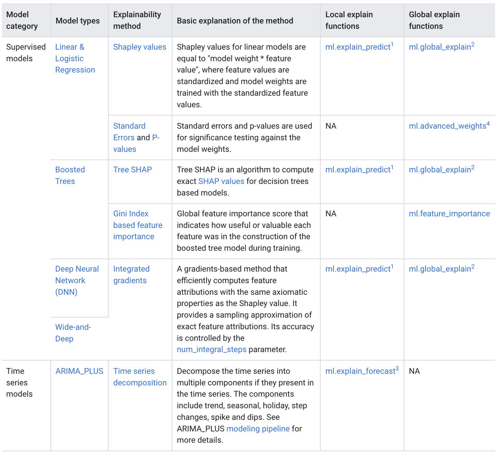
BigQuery Explainable AI applies to a variety of models, including supervised learning models for IID data and time series models. The documentation for BigQuery Explainable AI provides an overview of the different ways of applying explainability per model. Note that each explainability method has its own way of calculation (e.g. Shapley values), which are covered more in-depth in the documentation.
Examples with BigQuery Explainable AI
In this next section, we will show three examples of how to use BigQuery Explainable AI in different ML applications:
Regression models with BigQuery Explainable AI
Let’s use a boosted tree regression model to predict how much a taxi cab driver will receive in tips for a taxi ride, based on features such as number of passengers, payment type, total payment and trip distance. Then let’s use BigQuery Explainable AI to help us understand how the model made the predictions in terms of global explainability (which features were most important?) and local explainability (how did the model arrive at each prediction?).
The taxi trips dataset comes from the BigQuery public datasets and is publicly available in the table: bigquery-public-data.new_york_taxi_trips.tlc_yellow_trips_2018.
First, you can train a boosted tree regression model.
CREATE OR REPLACE MODEL bqml_tutorial.taxi_tip_regression_modelOPTIONS (model_type='boosted_tree_regressor',input_label_cols=['tip_amount'],max_iterations = 50,tree_method = 'HIST',subsample = 0.85,enable_global_explain = TRUE) ASSELECTvendor_id,passenger_count,trip_distance,rate_code,payment_type,total_amount,tip_amountFROM`bigquery-public-data.new_york_taxi_trips.tlc_yellow_trips_2018`WHERE tip_amount >= 0LIMIT 1000000
Now let’s do a prediction using ML.PREDICT, which is the standard way in BigQuery ML to make predictions without explainability.
SELECT *FROMML.PREDICT(MODEL bqml_tutorial.taxi_tip_regression_model,(SELECT"0" AS vendor_id,1 AS passenger_count,CAST(5.85 AS NUMERIC) AS trip_distance,"0" AS rate_code,"0" AS payment_type,CAST(55.56 AS NUMERIC) AS total_amount))

But you might wonder—how did the model generate this prediction of ~11.077?
BigQuery Explainable AI can help us answer this question. Instead of using ML.PREDICT, you use ML.EXPLAIN_PREDICT with an additional optional parameter top_k_features. ML.EXPLAIN_PREDICT extends the capabilities of ML.PREDICT by outputting several additional columns that explain how each feature contributes to the predicted value. In fact, since ML.EXPLAIN_PREDICT includes all the output from ML.PREDICT anyway, you may want to consider using ML.EXPLAIN_PREDICT every time instead.
SELECT *FROMML.EXPLAIN_PREDICT(MODEL bqml_tutorial.taxi_tip_regression_model,(SELECT"0" AS vendor_id,1 AS passenger_count,CAST(5.85 AS NUMERIC) AS trip_distance,"0" AS rate_code,"0" AS payment_type,CAST(55.56 AS NUMERIC) AS total_amount),STRUCT(6 AS top_k_features))
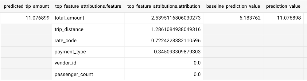
The way to interpret these columns is:
Σfeature_attributions + baseline_prediction_value = prediction_value
Let’s break this down. The prediction_value is ~11.077, which is simply the predicted_tip_amount. The baseline_prediction_value is ~6.184, which is the tip amount for an average instance. top_feature_attributions indicates how much each of the features contributes towards the prediction value. For example, total_amount contributes ~2.540 to the predicted_tip_amount.
ML.EXPLAIN_PREDICT provides local feature explainability for regression models. For global feature importance, see the documentation for ML.GLOBAL_EXPLAIN.
Classification models with BigQuery Explainable AI
Let’s use a logistic regression model to show you an example of BigQuery Explainable AI with classification models. We can use the same public dataset as before: bigquery-public-data.new_york_taxi_trips.tlc_yellow_trips_2018.
Train a logistic regression model to predict the bracket of the percentage of the tip amount out of the taxi bill.
CREATE OR REPLACE MODEL bqml_tutorial.taxi_tip_classification_modelOPTIONS(model_type='logistic_reg',input_label_cols=['tip_bucket'],enable_global_explain=true) ASSELECTvendor_id,passenger_count,trip_distance,rate_code,payment_type,total_amount,CASEWHEN tip_amount > total_amount*0.20 THEN '20% or more'WHEN tip_amount > total_amount*0.15 THEN '15% to 20%'WHEN tip_amount > total_amount*0.10 THEN '10% to 15%'ELSE '10% or less'END AS tip_bucketFROM`bigquery-public-data.new_york_taxi_trips.tlc_yellow_trips_2018`WHERE tip_amount >= 0LIMIT 1000000
Next, you can run ML.EXPLAIN_PREDICT to get both the classification results and the additional information for local feature explainability. For global explainability, you can use ML.GLOBAL_EXPLAIN. Again, since ML.EXPLAIN_PREDICT includes all the output from ML.PREDICT anyway, you may want to consider using ML.EXPLAIN_PREDICT every time instead.
SELECT *FROMML.EXPLAIN_PREDICT(MODEL bqml_tutorial.taxi_tip_classification_model,(SELECT"0" AS vendor_id,1 AS passenger_count,CAST(5.85 AS NUMERIC) AS trip_distance,"0" AS rate_code,"0" AS payment_type,CAST(55.56 AS NUMERIC) AS total_amount),STRUCT(6 AS top_k_features))
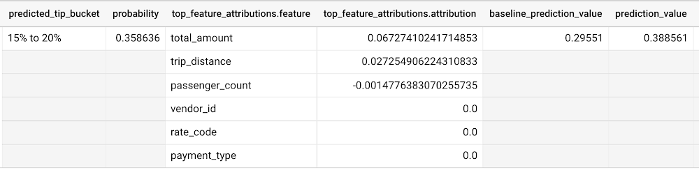
Similar to the regression example earlier, the formula is used to derive the prediction_value:
Σfeature_attributions + baseline_prediction_value = prediction_value
As you can see in the screenshot above, the baseline_prediction_value is ~0.296. total_amount is the most important feature in making this specific prediction, contributing ~0.067 to the prediction_value, though followed by trip_distance. The feature passenger_count contributes negatively to prediction_value by -0.0015. The features vendor_id, rate_code, and payment_type did not seem to contribute much to the prediction_value.
You may wonder why the prediction_value of ~0.389 doesn’t equal the probability value of ~0.359. The reason is that unlike for regression models, for classification models, prediction_value is not a probability score. Instead, prediction_value is the logit value (i.e., log-odds) for the predicted class, which you could separately convert to probabilities by applying the softmax transformation to the logit values. For example, a three-class classification has a log-odds output of [2.446, -2.021, -2.190]. After applying the softmax transformation, the probability of these class predictions is [0.9905, 0.0056, 0.0038].
Time-series forecasting models with BigQuery Explainable AI
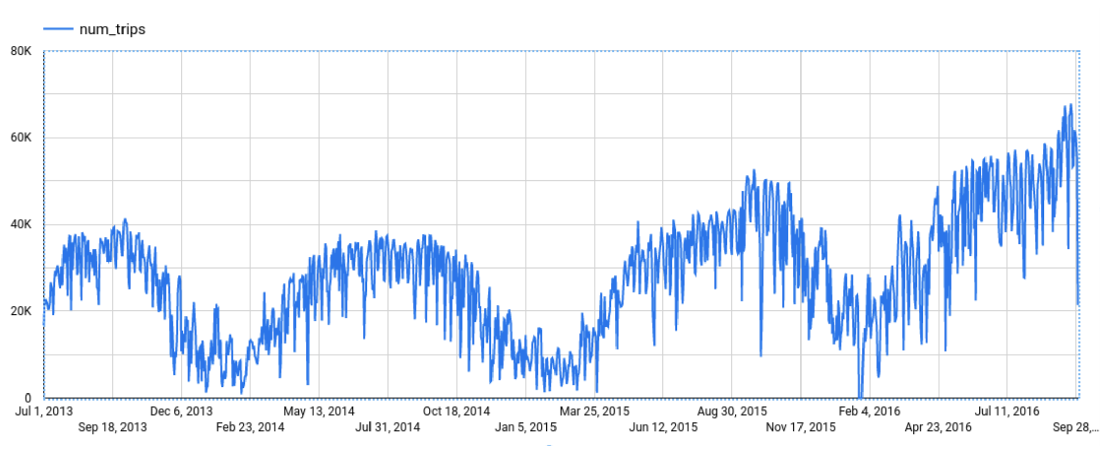
Explainable AI for forecasting provides more interpretability into how the forecasting model came to its predictions. Let’s go through an example of forecasting the number of bike trips in NYC using the new_york.citibike_trips public data in BigQuery.
You can train a time-series model ARIMA_PLUS:
CREATE OR REPLACE MODEL bqml_tutorial.nyc_citibike_arima_modelOPTIONS(model_type = 'ARIMA_PLUS',time_series_timestamp_col = 'date',time_series_data_col = 'num_trips',holiday_region = 'US') ASSELECTEXTRACT(DATE from starttime) AS date,COUNT(*) AS num_tripsFROM`bigquery-public-data.new_york.citibike_trips`GROUP BY dateNext, you can first try forecasting without explainability using ML.FORECAST:SELECT*FROMML.FORECAST(MODEL bqml_tutorial.nyc_citibike_arima_model,STRUCT(365 AS horizon, 0.9 AS confidence_level))
This function outputs the forecasted values and the prediction interval. Plotting it in addition to the input time series gives the following figure.
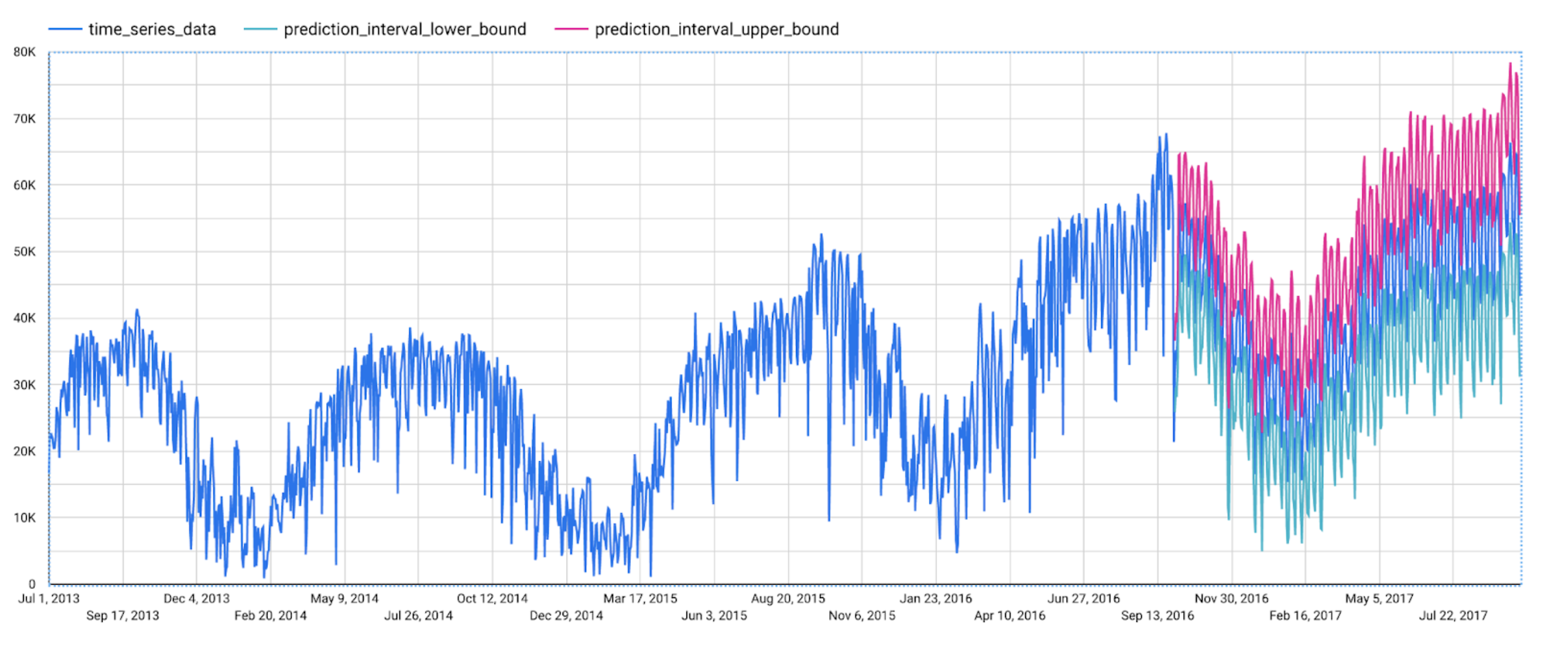
But how does the forecasting model arrive at its predictions? Explainability is especially important if the model ever generates unexpected results.
With ML.EXPLAIN_FORECAST, BigQuery Explainable AI provides extra transparency into the seasonality, trend, holiday effects, level (step) changes, and spikes and dips outlier removal. In fact, since ML.EXPLAIN_FORECAST includes all the output from ML.FORECAST anyway, you may want to consider using ML.EXPLAIN_FORECAST every time instead.
SELECT*FROMML.EXPLAIN_FORECAST(MODEL bqml_tutorial.nyc_citibike_arima_model,STRUCT(365 AS horizon, 0.9 AS confidence_level))
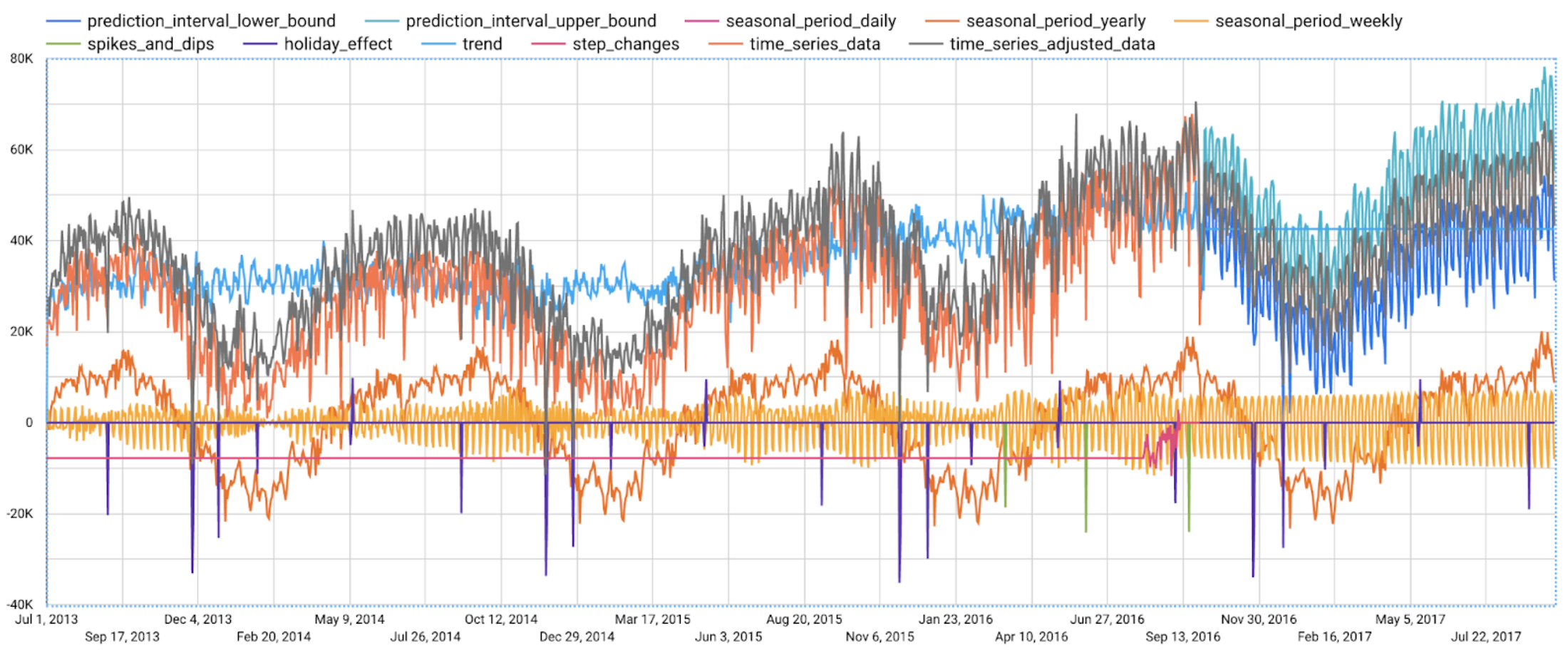
Compared to the previous figure which only shows the forecasting results, this figure shows much richer information to explain how the forecast is made.
First, it shows how the input time series is adjusted by removing the spikes and dips anomalies, and by compensating the level changes. That is:
time_series_adjusted_data = time_series_data - spikes_and_dips - step_changes
Second, it shows how the adjusted input time series is decomposed into different components such as both weekly and yearly seasonal components, holiday effect component and trend component. That is
time_series_adjusted_data = trend + seasonal_period_yearly + seasonal_period_weekly + holiday_effect + residual
Finally, it shows how these components are forecasted separately to compose the final forecasting results. That is:
time_series_data = trend + seasonal_period_yearly + seasonal_period_weekly + holiday_effect
For more information on these time series components, please see the documentation here.
Conclusion
With the GA of BigQuery Explainable AI, we hope you will now be able to interpret your machine learning models with ease.
Thanks to the BigQuery ML team, especially Lisa Yin, Jiashang Liu, Amir Hormati, Mingge Deng, Jerry Ye and Abhinav Khushraj. Also thanks to the Vertex Explainable AI team, especially David Pitman and Besim Avci.
IT Team Figures Out Easiest Way to Build Data Pipelines and Create ML Models

14076
Of your peers have already read this article.
5:15 Minutes
The most insightful time you'll spend today!
Building a strong brand in today’s hyper-competitive business environment takes vision. It also requires a flexible, easily managed approach to digital asset management (DAM), so marketing professionals and other stakeholders can easily share, store, track, and manipulate assets to build the brand.
Many of today’s leading companies, including JetBlue, Slack, TripAdvisor, Lyft, and HealthONE, rely on Brandfolder to deliver consistent, organized, and efficient brand experiences. Brandfolder provides an easy-to-use platform that can scale across an entire company with little end-user training, empowering customers to distribute digital assets wherever they are needed. Customers also gain much greater insight into how those assets are used, and how to use them more effectively in marketing campaigns and brand messaging.
“Google Cloud made it easy to build an ML platform to quickly iterate through different brand intelligence use cases and release data-driven product features into the Brandfolder platform.”
—Ajay Rajasekharan, Head of Data Science, Brandfolder
Brandfolder is constantly advancing its development efforts to introduce new data-driven features without complicating the user experience. Big data, artificial intelligence (AI), and machine learning (ML) are key to meeting customers’ unique business needs, and essential for Brandfolder to compete in the fast-moving DAM industry. To enhance these capabilities, Brandfolder sought a public cloud provider that could help it scale its data pipeline cost effectively while providing access to advanced AI technologies.
After graduating from the Techstars startup accelerator program in 2013, Brandfolder tried two other cloud providers before standardizing on Google Cloud Platform (GCP).
“We saw a difference with Google Cloud from the very beginning because the interactions felt like a strategic relationship,” says Jim Hanifen, Head of Product at Brandfolder. “Google gave us startup credits and a lot of face-to-face support, which we hadn’t experienced with other cloud providers. We decided to move our entire infrastructure to Google Cloud Platform.”
Building an ML platform for brand intelligence
After performing an initial lift-and-shift migration of virtual machines (VMs) onto Compute Engine, Brandfolder built an ML platform using GCP managed services to seamlessly deliver its data products. The platform leverages Cloud SQL, Cloud Storage as the data lake, Cloud Dataproc for cloud-native Apache Spark computing clusters, Cloud Composer as the batch job scheduler, Cloud Pub/Sub as the backbone data pipeline, Container Registry to store Docker images, and Google Kubernetes Engine (GKE) as the application orchestrator. Cloud Dataflow brings data into the data lake and into BigQuery for analysis.
“Google Cloud made it easy to build an ML platform to quickly iterate through different brand intelligence use cases and release data-driven product features into the Brandfolder platform,” says Ajay Rajasekharan, Head of Data Science at Brandfolder, who describes the architecture in a detailed blog. “We simply ingest raw application and event data on one end and output an ML service on the other.”
“Moving to Google Cloud Platform allows us to complete more sophisticated data analysis and ML models much faster, and at a much lower cost. We can create brand-specific ML models 12x faster and get them into production quickly to address our customers’ unique business needs.”
—Brett Nekolny, Head of Engineering, Brandfolder
For many general use cases, Brandfolder does not need to build custom ML models, and instead relies on pre-trained API models from GCP. For example, it uses Vision API and Video Intelligence API to auto-tag creative assets on import to enable fast, intuitive searches across images and videos. When more product- and brand-specific modeling is required to address unique customer use cases, Brandfolder builds and trains custom ML models using its GCP pipeline or Cloud AutoML, a suite of products built on Google transfer learning and neural architecture search technology. For example, if a Brandfolder customer makes different types of grills, Brandfolder can use AutoML Vision to train a model to recognize the different grills.
“Moving to Google Cloud Platform allows us to complete more sophisticated data analysis and ML models much faster, and at a much lower cost,” explains Brett Nekolny, Head of Engineering at Brandfolder. “We can create brand-specific ML models 12x faster and get them into production quickly to address our customers’ unique business needs.”
Industry-leading security and performance
Google Cloud’s security model helps Brandfolder give existing and prospective customers peace of mind that their data will be protected. Cloud Identity & Access Management (Cloud IAM) provides enterprise-grade access control, while Cloud Identity-Aware Proxy (Cloud IAP) enables remote users to work more securely without the hassles of a VPN client. GCP also isolates cloud resources into projects, making it easy to assign permissions and keep data and VMs organized and segregated.
“With Google Cloud, everything begins and ends with security, which makes things very easy for us,” says Jim. “If we’re under a security review, we can submit a Google security white paper. If a potential customer has security concerns, we tell them we are hosted on GCP, and those concerns go away.”
To give customers even better application performance for accessing their brand assets, Brandfolder uses Cloud Memorystore, an in-memory data store service for Redis, to cache data and provide sub-millisecond data access for production applications.
“It was much easier for us to use Cloud Memorystore versus running Redis on our compute instances,” says Brett. “The high availability, replication across zones, and automatic failover with no data loss are big for us.”
Global private network interconnects between Google Cloud and the Fastly content delivery network (CDN) dramatically reduce latency, allowing Brandfolder’s customers to deliver and update even very large creative assets quickly around the world.
“What’s beautiful about the relationship between Google and Fastly is that if one of our customers uploads a new version of an asset, we can propagate that out to Fastly, and the new version will automatically show up in all the places where it’s referenced,” says Brett.
“The ability to quickly solve problems with AI has a substantial impact on our revenue, and that’s more apparent every quarter. Few of our competitors are doing product- or brand-specific modeling because it takes a lot of time and resources. We overcame those hurdles with Google Cloud.”
—Jim Hanifen, Head of Product, Brandfolder
Improving employee and customer productivity
Brandfolder also uses Google solutions for real-time collaboration and productivity, using G Suite to connect employees with intuitive, cloud-based apps. Teams use Gmail, Calendar, Docs, Drive, Sheets, Slides, and Hangouts Meet every day to move the business forward. Many of Brandfolder’s customers are also G Suite users, and Brandfolder offers a plug-in that allows them to view their creative assets inside of Docs and pull images in as needed. Customers can also log into Brandfolder with their G Suite credentials, making the solution even easier to use.
“We’ve been using G Suite since the beginning, and it’s helped us collaborate efficiently to build a successful, growing company,” says Jim. “Our teams expect to have that kind of close collaboration, and everyone here enjoys the G Suite experience.”
Driving 99 percent annual business growth
With automated tagging and other innovative AI-based features, Brandfolder is helping customers locate and distribute assets faster. As a result, Brandfolder is building customer loyalty and increasing sales, growing its business by 99 percent year-over-year. Since moving to GCP, Brandfolder has been able to scale its analytics and data pipeline 50x without a corresponding increase in costs and has not had to expand its development team.
“The ability to quickly solve problems with AI has a substantial impact on our revenue, and that’s more apparent every quarter,” says Jim. “Few of our competitors are doing product- or brand-specific modeling because it takes a lot of time and resources. We overcame those hurdles with Google Cloud.”
A Comprehensive Guide for Understanding and Optimizing Your Dataflow Costs

1184
Of your peers have already read this article.
3:30 Minutes
The most insightful time you'll spend today!
Dataflow is the industry-leading platform that provides unified batch and streaming data processing capabilities, and supports a wide variety of analytics and machine learning use cases. It’s a fully managed service that comes with flexible development options (from Flex Templates and Notebooks to Apache Beam SDKs for Java, Python and Go), and a rich set of built-in management tools. It seamlessly integrates with not just Google Cloud products like Pub/Sub, BigQuery, Vertex AI, GCS, Spanner, and BigTable, but also third-party services like Kafka and AWS S3, to best meet your analytics and machine learning needs.
Dataflow’s adoption has ramped up in the past couple of years, and numerous customers now rely on Dataflow for everything from designing small proof of concepts, to large-scale production deployments. As customers are always trying to optimize their spend and do more with less, we naturally get questions related to cost optimization for Dataflow.
In this post, we’ve put together a comprehensive list of actions you can take to help you understand and optimize your Dataflow costs and business outcomes, based on our real-world experiences and product knowledge. We’ll start by helping you understand your current and near-term costs. We’ll then share how you can continuously evaluate and optimize your Dataflow pipelines over time. Let’s dive in!
Understand your current and near-term costs
The first step in most cost optimization projects is to understand your current state. For Dataflow, this involves the ability to effectively:
- Understand Dataflow’s cost components
- Predict the cost of potential jobs
- Monitor the cost of submitted jobs
Understanding Dataflow’s cost components
Your Dataflow job will have direct and indirect costs. Direct costs reflect resources consumed by your job, while indirect costs are incurred by the broader analytics/machine learning solution that your Dataflow pipeline enables. Examples of indirect costs include usage of different APIs invoked from your pipeline, such as:
- BigQuery Storage Read and Write APIs
- Cloud Storage APIs
- BigQuery queries
- Pub/Sub subscriptions and publishing, and
- Network egress, if any
Direct and indirect costs influence the total cost of your Dataflow pipeline. Therefore, it’s important to develop an intuitive understanding of both components, and use that knowledge to adopt strategies and techniques that help you arrive at a truly optimized architecture and cost for your entire analytics or machine learning solution. For more information about Dataflow pricing, see the Dataflow pricing page.
Predict the cost of potential jobs
You can predict the cost of a potential Dataflow job by initially running the job on a small scale. Once the small job is successfully completed, you can use its results to extrapolate the resource consumption of your production pipeline. Plugging those estimates into the Google Cloud Pricing Calculator should give you the predicted cost of your production pipeline. For more details about predicting the cost of potential jobs, see this (old, but very applicable) blog post on predicting the cost of a Dataflow job.
Monitor the cost of submitted jobs
You can monitor the overall cost of your Dataflow jobs using a few simple tools that Dataflow provides out of the box. Also, as you optimize your existing pipelines, possibly using recommendations from this blog post, you can monitor the impact of your changes on performance, cost, or other aspects of your pipeline that you care about. Handy techniques for monitoring your Dataflow pipelines include:
- Use metrics within the Dataflow UI to monitor key aspects of your pipeline.
- For CPU intensive pipelines, profile the pipeline to gain insight into how CPU resources are being used throughout your pipeline.
- Experience real-time cost control by creating monitoring alerts on Dataflow job metrics which ship out of the box, and that can be good proxies for the cost of your job. These alerts send real-time notifications once the metrics associated with a running pipeline exceeds a predetermined threshold. We recommend that you only do this for your critical pipelines, so you can avoid notification fatigue.
- Enable Billing Export into BiqQuery, and perform deep, ad-hoc analyses of your Dataflow costs that help you understand not just the key drivers of your costs, but also how these drivers are trending over time.
- Create a labeling taxonomy, and add labels to your Dataflow jobs that help facilitate cost attribution during the ad-hoc analyses of your Dataflow cost data using BigQuery. Check out this blog post for some great examples of how to do this.
- Run your Dataflow jobs using a custom Service Account. While this is great from a security perspective, it also has the added benefit of enabling the easy identification of APIs used by your Dataflow job.
Optimize your Dataflow costs
Once you have a good understanding of your Dataflow costs, the next step is to explore opportunities for optimization. Topics to be considered during this phase of your cost optimization journey include:
- Your optimization goals
- Key factors driving the cost of your pipeline
- Considerations for developing optimized batch and streaming pipelines
Let’s look at each of these topics in detail.
Goals
The goal of a cost optimization effort may seem obvious: “reduce my pipeline’s cost.” However, your business may have other priorities that have to be carefully considered and balanced with the cost reduction goal. From our conversations with customers, we have found that most Dataflow cost optimization programs have two main goals:
1. Reduce the pipeline’s cost
2. Continue meeting the service level agreements (SLAs) required by the business
Cost factors
Opportunities for optimizing the cost of your Dataflow pipeline will be based on the key factors driving your costs. While most of these factors will be identified through the process of understanding your current and near term costs, we have identified a set of frequently recurring cost factors, which we have grouped into three buckets: Dataflow configuration, performance, and business requirements.
Dataflow configuration includes factors like:
- Should your pipeline be streaming or batch?
- Are you using Dataflow services like Streaming Engine, or FlexRS?
- Are you using a suitable machine type and disk size?
- Should your pipeline be using GPUs?
- Do you have the right number of initial and maximum workers?
Performance includes factors like:
- Are your SDK versions (Java, Python, Go) up to date?
- Are you using IO connectors efficiently? One of the strengths of Apache Beam is a large library of IO connectors to different storage and queueing systems. Apache Beam IO connectors are already optimized for maximum performance. However, there may be cases where there are trade-offs between cost and performance. For example, BigQueryIO supports several write methods, each of them with somewhat different performance and cost characteristics. For more details, see slides 19 – 22 of the Beam Summit session on cost optimization.
- Are you using efficient coders? Coders affect the size of the data that needs to be saved to disk or transferred to a dedicated shuffle service in the intermediate pipeline stages, and some coders are more efficient than others. Metrics like total shuffle data processed and total streaming data processed can help you identify opportunities for using more efficient coders. As a general rule, you should consider whether the data that appears in your pipeline contains redundant data that can be eliminated by both filtering out unused columns as early as possible, and using efficient coders such as AvroCoder or RowCoder. Also, remember that if stages of your pipeline are fused, the coders in the intermediate steps become irrelevant.
- Do you have sufficient parallelism in your pipeline? The execution details tab, and metrics like processing parallelism keys can help you determine whether your pipeline code is taking full advantage of Apache Beam’s ability to do massively parallel processing (for more details, see parallelism). For example, if you have a transform which outputs a number of records for each input record (“high fan-out transform”) and the pipeline is automatically optimized using Dataflow fusion optimization, the parallelism of the pipeline can be suboptimal, and may benefit from preventing fusion. Another area to watch for is “hot keys.” This blog discusses this topic in great detail.
- Are your custom transforms efficient? Job monitoring techniques like profiling your pipeline and viewing relevant metrics can help you catch and correct your inefficient use of custom transforms. For example, if your Java transform needs to check if the data matches a certain regular expression pattern, then compiling that pattern in the setup method and doing the matching using the precompiled pattern in the “process element” method is much more efficient. The simpler, but inefficient alternative is to use the String.matches() call in the “process element” method, which will have to compile the pattern every time. Another consideration regarding custom transforms is that grouping elements for external service calls can help you prepare optimal request batches for external API calls. Finally, transforms that perform multi-step operations (for example, calls to external APIs that require extensive processes for creating and closing the client for the API) can often benefit from splitting these operations, and invoking them in different methods of the ParDo (for more details, see ParDo life cycle).
- Are you doing excessive logging? Logs are great. They help with debugging, and can significantly improve developer productivity. On the other hand, excessive logging can negatively impact your pipeline’s performance.
Business requirements can also influence your pipeline’s design, and increase costs. Examples of such requirements include:
- Low end-to-end ingest latency
- Extremely high throughput
- Processing late arriving data
- Processing streaming data spikes
Considerations for developing optimized data pipelines
From our work with customers, we have compiled a set of guidelines that you can easily explore and implement to effectively optimize your Dataflow costs. Examples of these guidelines include:
Batch and streaming pipelines:
- Consider keeping your Dataflow job in the same region as your IO source and destination services.
- Consider using GPUs for specialized use cases like deep-learning inference.
- Consider specialized machine types for memory- or compute-intensive workloads.
- Consider setting the maximum number of workers for your Dataflow job.
- Consider using custom containers to pre-install pipeline dependencies, and speed up worker startup time.
- Where necessary, tune the memory of your worker VMs.
- Reduce your number of test and staging pipelines, and remember to stop pipelines that you no longer need.
Batch pipelines:
- Consider FlexRS for use cases that have start time and run time flexibility.
- Run fewer pipelines on larger datasets. Starting and stopping a pipeline incurs some cost, and processing a very small dataset in a batch pipeline can be inefficient.
- Consider defining the maximum duration for your jobs, so you can eliminate runaway jobs, which keep running without delivering value to your business.
Summary
In this post, we introduced you to a set of knowledge and techniques that can help you understand the current and near-term costs associated with your Dataflow pipelines. We also shared a series of considerations that can help you optimize your Dataflow pipelines, not just for today, but also as your business evolves over time. We shared lots of resources with you, and hope that you find them useful. We look forward to hearing about the savings and innovative solutions that you are able to deliver for your customers and your business.

3466
Of your peers have already downloaded this article
10:30 Minutes
The most insightful time you'll spend today!
As organizations look to revolutionize how they analyze and utilize data, modernizing the data-centric technology stack is critical to success.
Today, the traditional stack poses several challenges—too many steps, too many tools, and too many integrations—all leading to operational complexity, time delays, and high cost. Simplifying the data pipeline, data lifecycle, and data stack offers organizations improved efficiency as well as cost savings, and provides them more value by freeing up resources to focus on deriving insight through the analysis of data.
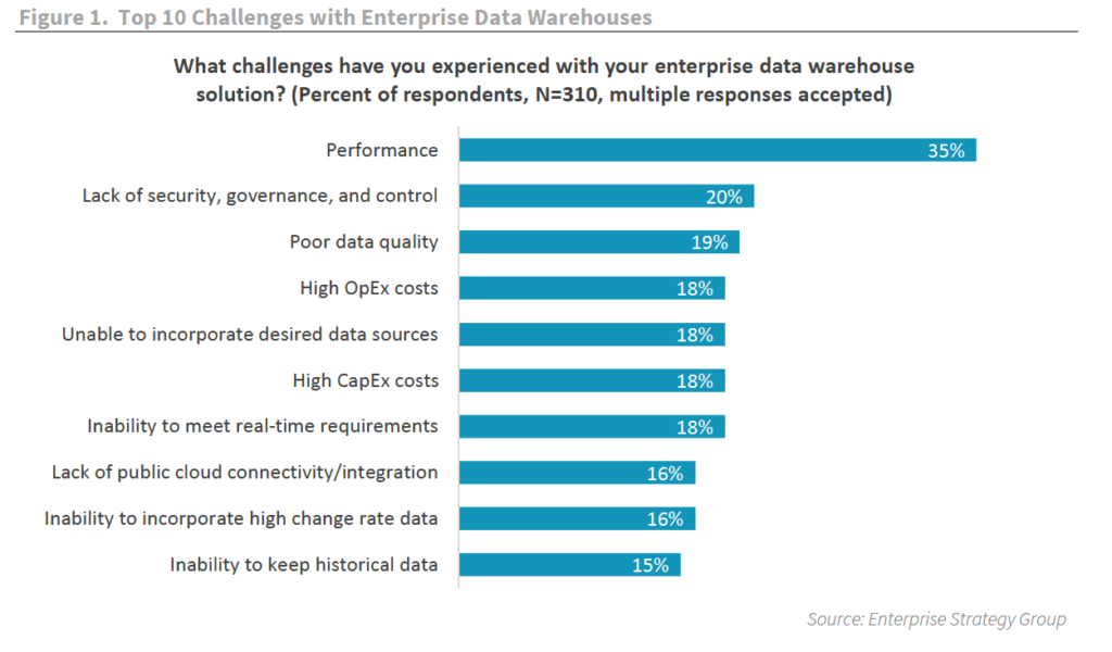
As organizations begin to transform their approach to analytics, modernizing the analytics stack is a top priority.
To address both the data supply and data demand, data teams must look for ways to simplify and optimize the data pipeline. That means transitioning traditional solutions, like data warehouses and business intelligence tools, to modern architectures built with scalability, agility, and availability in mind.
And what follows with a modernized stack is an ideal data experience rich in actionable insight, API-driven application integration, and the ability to address the real-time needs of a dynamic business.
To find out the advantages to modernizing data warehouses and how this can be accomplished, download, ESG’s report: Modernize the Data Stack to Transform the Data Experience.
3138
Of your peers have already watched this video.
24:30 Minutes
The most insightful time you'll spend today!
How to Build a Global Marketing Data Hub
Data-driven marketing ensures that the right message is reaching the right customer at the right time through the right channel. However if an organization’s data resides in multiple systems and platforms it hampers its ability to deliver truly global data-driven campaigns, attribution analysis, and reporting.
See how Cloud Data Fusion with its growing plugins ecosystem can be leveraged to integrate multiple disparate data sources to build a comprehensive Marketing Data Warehouse. Learn how Cloud Data Fusion helped global CPG organizations build their Marketing DW.
Prateek Duble, Data Analytics Specialist, Google Cloud and Bhooshan Mogal, Product Manager, Cloud Data Fusion, Google Cloud, cover:
- How enterprises can build a robust global marketing data warehouse with Google Cloud including the business needs and technical challenge they encounter while building the holistic marketing data warehouses.
- How Cloud Data Fusion, Google Cloud Platform’s data ingestion and integration product, delivers critical capabilities to accelerate an enterprises’ journey to building marketing data warehouse.
- A reference architecture with Google Cloud products that shows how easily and quickly you can build marketing data warehouse in Google Cloud.
- A recent case study of a CPG business who built their marketing data warehouse with Google Cloud Platform.
This presentation also includes recent product launch announcements.
3172
Of your peers have already watched this video.
23:00 Minutes
The most insightful time you'll spend today!
Best Practices from Experts to Maximize BigQuery Performance (Featuring Twitter)
If you have made the decision to run your data analytics on BigQuery’s serverless platform, you are in good company.
Now, as you deploy complex workloads on your data, you want to be able to maximize the performance of all data operations from data loading to data analytics.
In this video Jagan Athreya, Product Manager, Google Cloud and Gary Steelman, Senior Software Engineer, Twitter discuss the best practices from speeding up your data ingest into BigQuery to learning the tips and tricks from the BigQuery engineering team to maximize query performance of your data warehouse.
The session is roughly divided into five areas:
- The architecture that enables the performance of BigQuery
- An example of a typical query
- How to write fast and efficient queries
- The best way to ingest data
- Twitter case study
More Relevant Stories for Your Company
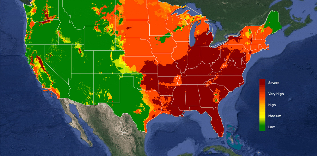
Predictive Model Built on Google Cloud Helps You Get a 7-day Mosquito Forecast Report!
Mosquitoes aren’t just the peskiest creatures on Earth; they infect more than 700 million people a year with dangerous diseases like Zika, Malaria, Dengue Fever, and Yellow Fever. Prevention is the best protection, and stopping mosquito bites before they happen is a critical step. SC Johnson—a leading developer and manufacturer

How Do You Cut Costs and Improve Staff Productivity, and Business Visibility? Ascend Money Has an Answer
Hundreds of millions of residents of South East Asia have only limited access to banking and finance services. However, help is at hand. One of South East Asia's largest fintech businesses, Ascend Money is using digital technologies to realize its mission of enabling as many people as possible to access

AirAsia Turns to Google Cloud to refine Pricing, Increase Revenue, and Improve Customer Experience
AirAsia needed a platform incorporating products that could capture, process, analyze, and report on data, while delivering value for money and meeting its speed and availability requirements. The airline also wanted to minimise infrastructure management and system administration demands on its technology team members. The airline conducted a proof of

How Google Cloud Helps SAP Admins Create Scalable, Secure Networks
SAP forms the critical backbone of thousands of enterprises, supporting critical business functions such as finance, supply chain, warehouse management, and more. Google Cloud provides a highly scalable and resilient infrastructure to run such workloads and offers tools, such as Smart Analytics and Machine Learning that can accelerate your organization’s digital transformation. In fact, a
