





Recommendations for Modelling SAP Data inside BigQuery
8404
Of your peers have already read this article.
4:00 Minutes
The most insightful time you'll spend today!
Over the past few years, many organizations have experienced the benefits of migrating their SAP solutions to Google Cloud. But this migration can do more than reduce IT maintenance costs and make data more secure. By leveraging BigQuery, SAP customers can complement their SAP investments and gain fresh insights by consolidating enterprise data and easily extending it with powerful datasets and machine learning from Google.
BigQuery is a leading cloud data warehouse, fully managed and serverless, and allows for massive scale, supporting petabyte-scale queries at super-fast speeds. It can easily combine SAP data with additional data sources, such as Google Analytics or Salesforce, and its built-in machine learning lets users operationalize machine learning models using standard SQL — all at a comparatively low cost.
If your SAP-powered organization is looking to supercharge its analytics with the strength of BigQuery, read on for considerations and recommendations for modeling with SAP data. These guidelines are based on our real-world implementation experience with customers and can serve as a roadmap to the analytics capabilities your business needs.
Considerations for data replication
Like most technology journeys, this one should start with a business objective. Keeping your intended business value and goals in mind is critical to making the right decisions in the early steps of the design process.
When it comes to replicating the data from an SAP system into BigQuery, there are multiple ways to do it successfully. Decide which method will work best for your organization by answering these questions:
- Does your business need real-time data? Will you need to time travel into past data?
- Which external datasets will you need to join with the replicated data?
- Are the source structures or business logic likely to change? Will you be migrating the SAP source systems any time soon? For instance, will you be moving from SAP ECC to SAP S/4HANA?
You’ll also need to determine whether replication should be done on a table-by-table basis or whether your team can source from pre-built logic. This decision, along with other considerations such as licensing, will influence which replication tool you should use.
Replicating on a table-by-table basis
Replicating tables, especially standard tables in their raw form, allows sources to be reused and ensures more stability of the source structure and functional output. For example, the SAP table for sales order headers (VBAK) is very unlikely to change its structure across different versions of SAP, and the logic that writes to it is also unlikely to change in a way that affects a replicated table.
Something else to consider: Reconciliation between the source system and the landing table in BigQuery is linear when comparing raw tables, which helps avoid issues in consolidation exercises during critical business processes, such as period-end closing. Since replicated tables aren’t aggregated or subject to process-specific data transformation, the same replicated columns can be reused in different BigQuery views. You can, for instance, replicate the MARA table (the material master) once and use it in as many models as needed.
Replicating pre-built logic
If you replicate pre-built models, such as those from SAP extractors or CDS views, you don’t need to build the logic in BigQuery, since you’re using existing logic. Some of these extraction objects have embedded delta mechanisms, which may complement a replication tool that can’t handle deltas. This will save initial development time, but it can also lead to challenges if you create new columns, or if customizations or upgrades change the logic behind the extraction.
It’s also important to note that different extraction processes may transform and load the same source columns multiple times, which creates redundancy in BigQuery and can lead to higher maintenance needs and costs. However, replicating pre-built models may still be a good choice, since doing so can be especially useful for logic that tends to be immutable, such as flattening a hierarchy, or logic that is highly complex.
How you approach replication will also depend on your long-term plans and other key factors — for example, the availability (and curiosity) of your developers, and the time or effort they can put into applying their SQL knowledge to a new data warehouse.
With either replication approach, bear in mind when designing your replication process that BigQuery is meant to be an append-always database — so post-processing of data and changes will be required in both cases.
Processing data changes
The replication tool you choose will also determine how data changes are captured (known as CDC – change data capture). If the replication tool allows for it (for example as SAP SLT does) the same patterns described in the CDC with BigQuery documentation also apply to SAP data.
Because some data, like transactions, are known to be less static than others (e.g., master data), you need to decide what should be scanned in real time, what will require immediate consistency, and what can be processed in batches to manage costs. This decision will be based on the reporting needs from the business.
Consider the SAP table BUT000, containing our example master data for business partners, where we have replicated changes from an SAP ERP system:
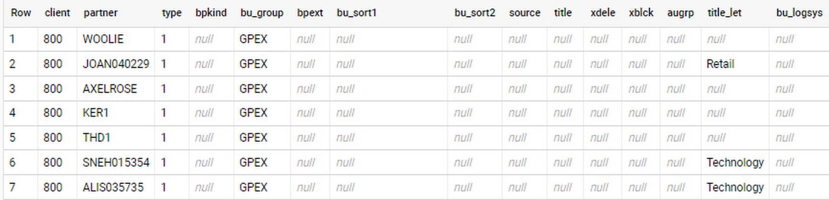
In an append-always replication in BigQuery, all updates are received as new records. For example, deleting a record in the source will be represented as a new record in BigQuery with a deletion flag. This applies to whether the records are coming from raw tables like BUT000 itself or pre-aggregated data, as from a BW extractor or a CDS view.
Let’s take a closer look at data coming particularly from the partners “LUCIA” and “RIZ”. The operation flag tells us whether the new record in BigQuery is an insert (I), update (U) or deletion (D), while the timestamps help us identify the latest version of our business partner.
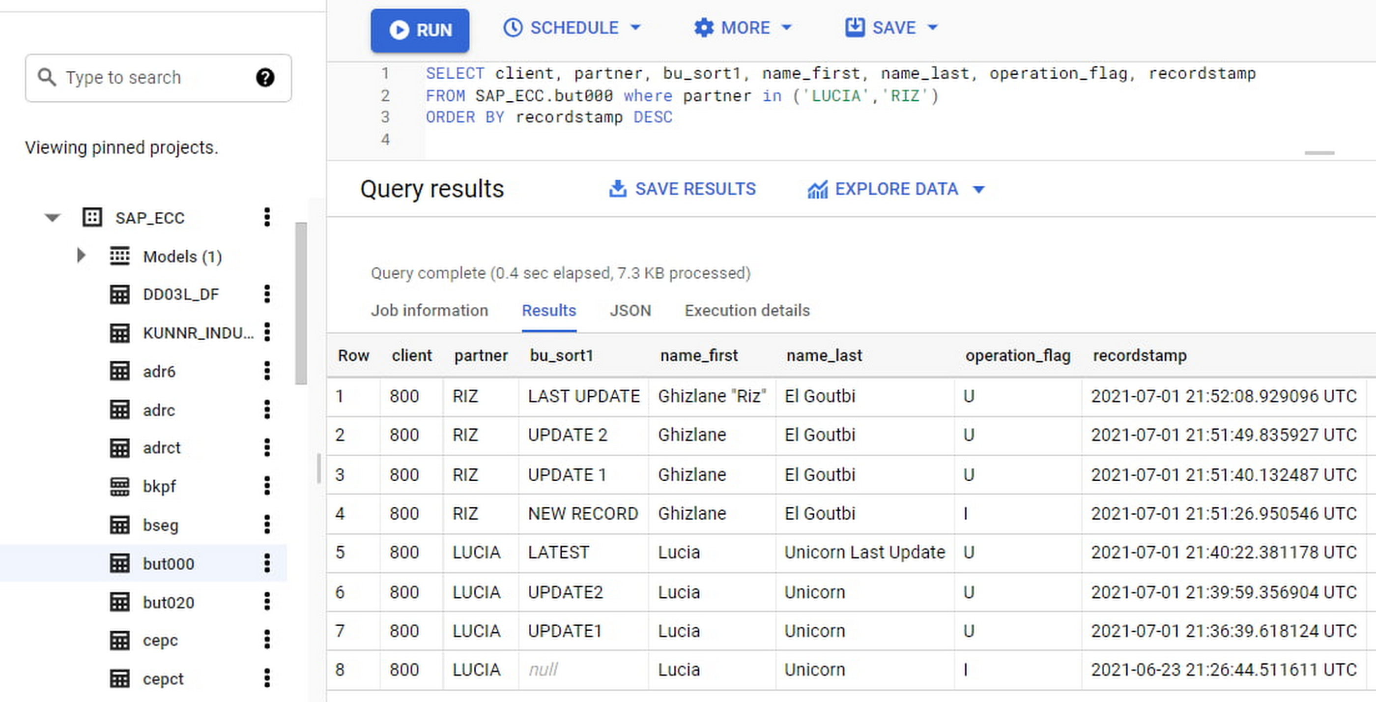
If we want to find the latest updated record for the partners LUCIA and RIZ, this is what the query would look like:
SELECT partner,ARRAY_AGG(i1 ORDER BY i1.recordstamp DESC LIMIT 1) AS rowFROM SAP_ECC.but000 i1WHERE partner in ('LUCIA','RIZ')GROUP BY partner
With the following result:
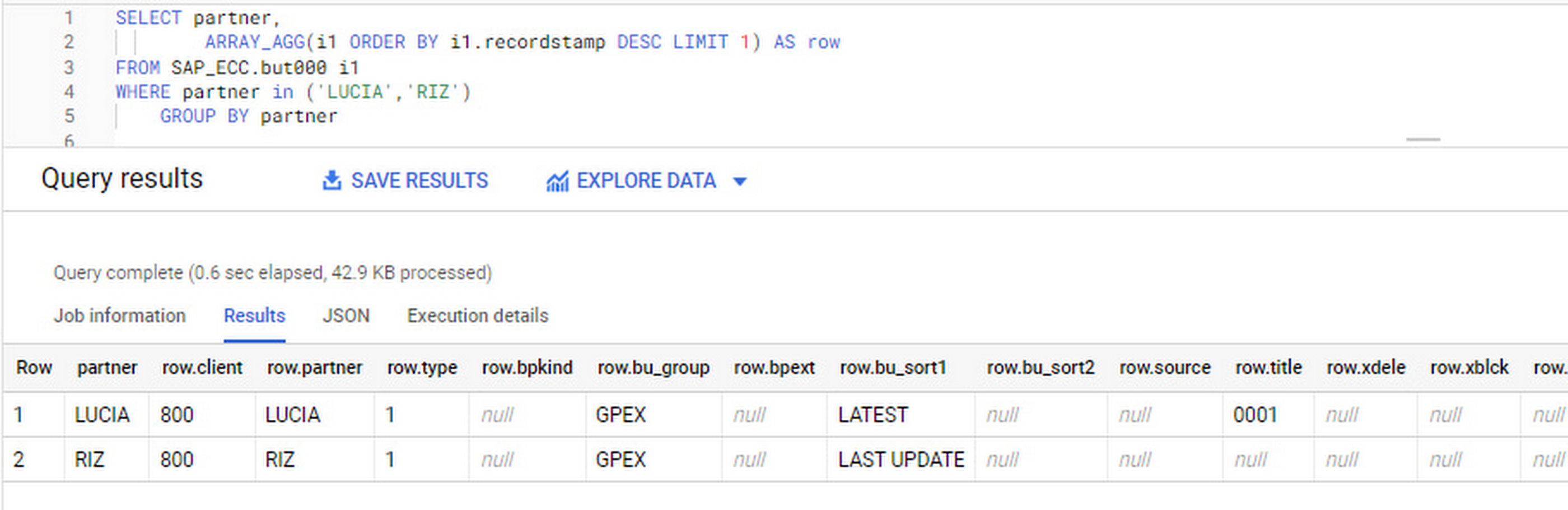
After identifying stale records for “LUCIA” and “RIZ” business partners, we can proceed to deleting all stale records for “LUCIA” if we do not want to retain the history. In this example, we are using a different table to which the same replication has been done, for the purpose of comparison and to check that all stale records have been deleted for the selection made and that we only kept last updated records. For example:
DELETE SAP_HANA.but000 i1WHEREi1.recordstamp < TIMESTAMP_SUB(CURRENT_TIMESTAMP(), INTERVAL 3 HOUR) ANDi1.recordstamp < (SELECT MAX(recordstamp) FROM SAP_HANA.but000 i2WHEREi1.partner = i2.partnerand partner="LUCIA")
You can also use the following query to retrieve stale records for “LUCIA” partner before moving forward with deletion
SELECT partner, operation_flag, recordstamp FROM SAP_HANA.but000 i1WHEREi1.recordstamp < TIMESTAMP_SUB(CURRENT_TIMESTAMP(), INTERVAL 3 HOUR)ANDi1.recordstamp < (SELECT MAX(recordstamp) FROM SAP_HANA.but000 i2WHEREi1.partner = i2.partnerand partner="LUCIA")
Which produces all of the records, except the latest update:

Partitioning and clustering
To limit the number of records scanned in a query, save on cost and achieve the best performance possible, you’ll need to take two important steps: determine partitions and create clusters.
Partitioning
A partitioned table is one that’s divided into segments, called partitions, which make it easier to manage and query your data. Dividing a large table into smaller partitions improves query performance and controls costs because it reduces the number of bytes read by a query.
You can partition BigQuery tables by:
- Time-unit column: Tables are partitioned based on a “timestamp,” “date,” or “datetime” column in the table.
- Ingestion time: Tables are partitioned based on the timestamp recorded when BigQuery ingested the data.
- Integer range: Tables are partitioned based on an integer column.
Partitions are enabled when the table is created, as in the example below. A great tip is to always include the partition filter as shown on the left-hand side of the query.

Clustering
Clustering can be created on top of partitioned tables by applying the fields that are likely to be used for filtering. When you create a clustered table in BigQuery, the table data is automatically organized based on the contents of one or more of the columns in the table’s schema. The columns you specify are then used to colocate related data.
Clustering can improve the performance of certain query types — for example, queries that use filter clauses or that aggregate data. It makes a lot of sense to use them for large tables such as ACDOCA, the table for accounting documents in SAP S/4HANA. In this case, the timestamp could be used for partitioning, and common filtering fields such as the ledger, company code, and fiscal year could be used to define the clusters.
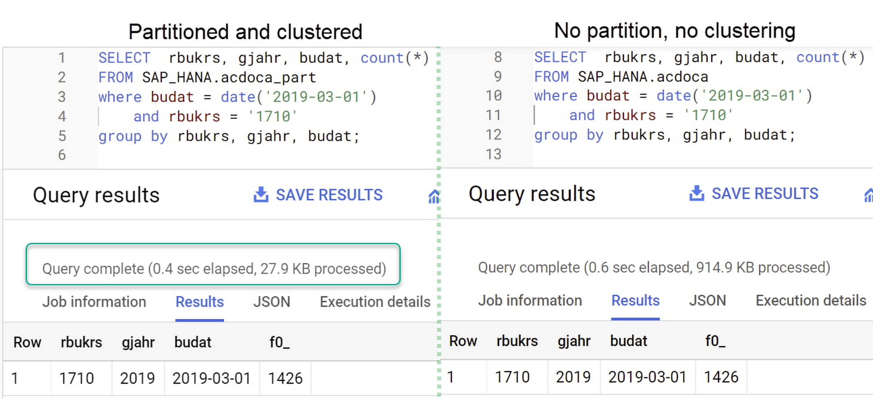
A great feature is that BigQuery will also periodically recluster the data automatically.
Materialized views
In BigQuery, materialized views are precomputed views that periodically cache the results of a query for better performance and efficiency. BigQuery uses precomputed results from materialized views and, whenever possible, reads only the delta changes from the base table to compute up-to-date results quickly. Materialized views can be queried directly or can be used by the BigQuery optimizer to process queries to the base table.
Queries that use materialized views are generally completed faster and consume fewer resources than queries that retrieve the same data only from the base table. If workload performance is an issue, materialized views can significantly improve the performance of workloads that have common and repeated queries. While materialized views currently only support single tables, they are very useful common and frequent aggregations like stock levels or order fulfillment.
Further tips on performance optimization while creating select statements can be found in the documentation for optimizing query computation.
Deployment pipeline and security
For most of the work you’ll do in BigQuery, you’ll normally have at least two delivery pipelines running — one for the actual objects in BigQuery and the other to keep the data staging, transforming, and updated as intended within the change-data-capture flows. Note that you can use most existing tools for your Continuous Integration / Continuous Deployment (CI/CD) pipeline — one of the benefits of using an open system like BigQuery. But, if your organization is new to CI/CD pipelines, this is a great opportunity to gradually gain experience. A good place to start is to read our guide for setting up a CI/CD pipeline for your data-processing workflow.
When it comes to access and security, most end-users will only have access to the final version of the BigQuery views. While row and column-level security can be applied, as in the SAP source system, separation of concerns can be taken to the next level by splitting your data across different Google Cloud projects and BigQuery datasets. While it’s easy to replicate data and structures across your datasets, it’s a good idea to define the requirements and naming conventions early in the design process so you set it up properly from the start.
Start driving faster and more insightful analytics
The best piece of advice we can give you is this: Try it yourself. Anyone with SQL knowledge can get started using the free BigQuery tier. New customers get $300 in free credits to spend on Google Cloud during the first 90 days. All customers get 10 GB storage and up to 1 TB queries/month, completely free of charge. In addition to discovering the massive processing capabilities, embedded machine learning, multiple integration tools, and cost benefits, you’ll soon discover how BigQuery can simplify your analytics tasks.
If you need additional assistance, our Google Cloud Professional Services Organization (PSO) and Customer Engineers will be happy to help show you the best path forward for your organization. For anything else, contact us at cloud.google.com/contact.
10146
Of your peers have already watched this video.
1:00 Minutes
The most insightful time you'll spend today!
Predict User Churn on Gaming Apps with Google Analytics Data using BigQuery ML
User retention can be a major challenge for mobile game developers. According to the Mobile Gaming Industry Analysis in 2019, most mobile games only see a 25% retention rate for users after the first day. To retain a larger percentage of users after their first use of an app, developers can take steps to motivate and incentivize certain users to return. But to do so, developers need to identify the propensity of any specific user returning after the first 24 hours.
In this blog post, we will discuss how you can use BigQuery ML to run propensity models on Google Analytics 4 data from your gaming app to determine the likelihood of specific users returning to your app.
You can also use the same end-to-end solution approach in other types of apps using Google Analytics for Firebase as well as apps and websites using Google Analytics 4. To try out the steps in this blogpost or to implement the solution for your own data, you can use this Jupyter Notebook.
Using this blog post and the accompanying Jupyter Notebook, you’ll learn how to:
- Explore the BigQuery export dataset for Google Analytics 4
- Prepare the training data using demographic and behavioural attributes
- Train propensity models using BigQuery ML
- Evaluate BigQuery ML models
- Make predictions using the BigQuery ML models
- Implement model insights in practical implementations
Google Analytics 4 (GA4) properties unify app and website measurement on a single platform and are now default in Google Analytics. Any business that wants to measure their website, app, or both, can use GA4 for a more complete view of how customers engage with their business. With the launch of Google Analytics 4, BigQuery export of Google Analytics data is now available to all users. If you are already using a Google Analytics 4 property, you can follow this guide to set up exporting your GA data to BigQuery.
Once you have set up the BigQuery export, you can explore the data in BigQuery. Google Analytics 4 uses an event-based measurement model. Each row in the data is an event with additional parameters and properties. The Schema for BigQuery Export can help you to understand the structure of the data.
In this blogpost, we use the public sample export data from an actual mobile game app called “Flood It!” (Android, iOS) to build a churn prediction model. But you can use data from your own app or website.
Here’s what the data looks like. Each row in the dataset is a unique event, which can contain nested fields for event parameters.
SELECT *FROM `firebase-public-project.analytics_153293282.events_*`TABLESAMPLE SYSTEM (1 PERCENT)
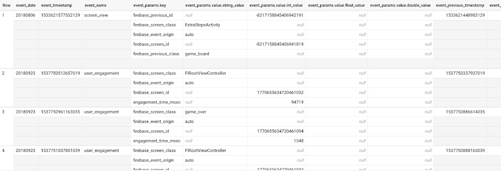
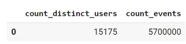
This dataset contains 5.7M events from over 15k users.
SELECTCOUNT(DISTINCT user_pseudo_id) as count_distinct_users,COUNT(event_timestamp) as count_eventsFROM`firebase-public-project.analytics_153293282.events_*
Our goal is to use BigQuery ML on the sample app dataset to predict propensity to user churn or not churn based on users’ demographics and activities within the first 24 hours of app installation.
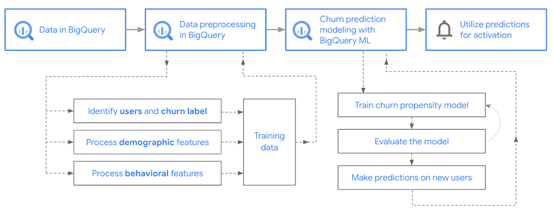
In the following sections, we’ll cover how to:
- Pre-process the raw event data from GA4
- Identify users & the label feature
- Process demographic features
- Process behavioral features
- Train classification model using BigQuery ML
- Evaluate the model using BigQueryML
- Make predictions using BigQuery ML
- Utilize predictions for activation
Pre-process the raw event data
You cannot simply use raw event data to train a machine learning model as it would not be in the right shape and format to use as training data. So in this section, we’ll go through how to pre-process the raw data into an appropriate format to use as training data for classification models.
This is what the training data should look like for our use case at the end of this section:
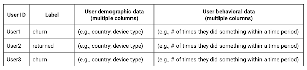
Notice that in this training data, each row represents a unique user with a distinct user ID (user_pseudo_id).
Identify users & the label feature
We first filtered the dataset to remove users who were unlikely to return the app anyway. We defined these ‘bounced’ users as ones who spent less than 10 mins with the app. Then we labeled all remaining users:
- churned: No event data for the user after 24 hours of first engaging with the app.
- returned: The user has at least one event record after 24 hours of first engaging with the app.
For your use case, you can have a different definition of bounce and churning. Also you can even try to predict something else other than churning, e.g.:
- whether a user is likely to spend money on in-game currency
- likelihood of completing n-number of game levels
- likelihood of spending n amount of time in-game etc.
In such cases, label each record accordingly so that whatever you are trying to predict can be identified from the label column.
From our dataset, we found that ~41% users (5,557) bounced. However, from the remaining users (8,031), ~23% (1,883) churned after 24 hours:
SELECTbounced,churned,COUNT(churned) as count_usersFROMbqmlga4.returningusersGROUP BY 1,2ORDER BY bounced
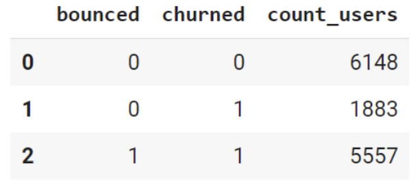
To create these bounced and churned columns, we used the following snippet of SQL code.
...#churned = 1 if last_touch within 24 hr of app installation, else 0IF (user_last_engagement < TIMESTAMP_ADD(user_first_engagement,INTERVAL 24 HOUR),1,0 ) AS churned,#bounced = 1 if last_touch within 10 min, else 0IF (user_last_engagement <= TIMESTAMP_ADD(user_first_engagement,INTERVAL 10 MINUTE),1,0 ) AS bounced,...
You can view the Jupyter Notebook for the full query used for materializing the bounced and churned labels.
Process demographic features
Next, we added features both for demographic data and for behavioral data spanning across multiple columns. Having a combination of both demographic data and behavioral data helps to create a more predictive model.
We used the following fields for each user as demographic features:
geo.countrydevice.operating_systemdevice.language
A user might have multiple unique values in these fields — for example if a user uses the app from two different devices. To simplify, we used the values from the very first user engagement event.
CREATE OR REPLACE VIEW bqmlga4.user_demographics AS (WITH first_values AS (SELECTuser_pseudo_id,geo.country as country,device.operating_system as operating_system,device.language as language,ROW_NUMBER() OVER (PARTITION BY user_pseudo_id ORDER BY event_timestamp DESC) AS row_numFROM `firebase-public-project.analytics_153293282.events_*`WHERE event_name="user_engagement")SELECT * EXCEPT (row_num)FROM first_valuesWHERE row_num = 1 #first engagement);
Process behavioral features
There is additional demographic information present in the GA4 export dataset, e.g. app_info, device, event_params, geo etc. You may also send demographic information to Google Analytics through each hit via user_properties. Furthermore, if you have first-party data on your own system, you can join that with the GA4 export data based on user_ids.
To extract user behavior from the data, we looked into the user’s activities within the first 24 hours of first user engagement. In addition to the events automatically collected by Google Analytics, there are also the recommended events for games that can be explored to analyze user behavior. For our use case, to predict user churn, we counted the number of times the follow events were collected for a user within 24 hours of first user engagement:
user_engagementlevel_start_quickplaylevel_end_quickplaylevel_complete_quickplaylevel_reset_quickplaypost_scorespend_virtual_currencyad_rewardchallenge_a_friendcompleted_5_levelsuse_extra_steps
The following query shows how these features were calculated:
WITHevents_first24hr AS (SELECTe.*FROM`firebase-public-project.analytics_153293282.events_*` eJOINbqmlga4.returningusers rONe.user_pseudo_id = r.user_pseudo_idWHERETIMESTAMP_MICROS(e.event_timestamp) <= r.ts_24hr_after_first_engagement)SELECTuser_pseudo_id,SUM(IF(event_name = 'user_engagement', 1, 0)) AS cnt_user_engagement,# ... repeated for all behavior data ...SUM(IF(event_name = 'use_extra_steps', 1, 0)) AS cnt_use_extra_steps,FROMevents_first24hrGROUP BY1
View the notebook for the query used to aggregate and extract the behavioral data. You can use different sets of events for your use case. To view the complete list of events, use the following query:
SELECTevent_name,COUNT(event_name) as event_countFROM`firebase-public-project.analytics_153293282.events_*`GROUP BY 1ORDER BYevent_count DESC
After this we combined the features to ensure our training dataset reflects the intended structure. We had the following columns in our table:
- User ID:
user_pseudo_id
- Label:
churned
- Demographic features
countrydevice_osdevice_language
- Behavioral features
cnt_user_engagementcnt_level_start_quickplaycnt_level_end_quickplaycnt_level_complete_quickplaycnt_level_reset_quickplaycnt_post_scorecnt_spend_virtual_currencycnt_ad_rewardcnt_challenge_a_friendcnt_completed_5_levelscnt_use_extra_stepsuser_first_engagement
At this point, the dataset was ready to train the classification machine learning model in BigQuery ML. Once trained, the model will output a propensity score between churn (churned=1) or return (churned=0) indicating the probability of a user churning based on the training data.
Train classification model
When using the CREATE MODEL statement, BigQuery ML automatically splits the data between training and test. Thus the model can be evaluated immediately after training (see the documentation for more information).
For the ML model, we can choose among the following classification algorithms where each type has its own pros and cons:
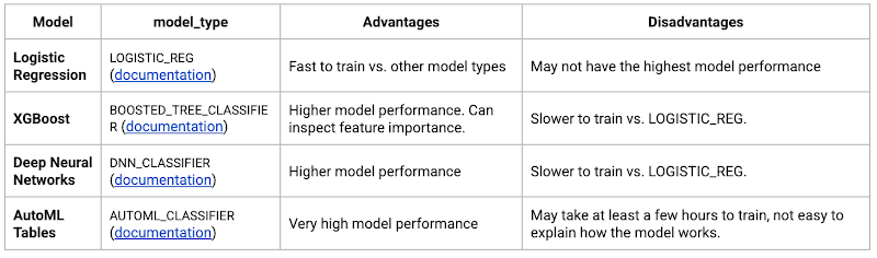
Often logistic regression is used as a starting point because it is the fastest to train. The query below shows how we trained the logistic regression classification models in BigQuery ML.
CREATE OR REPLACE MODEL bqmlga4.churn_logregTRANSFORM(EXTRACT(MONTH from user_first_engagement) as month,EXTRACT(DAYOFYEAR from user_first_engagement) as julianday,EXTRACT(DAYOFWEEK from user_first_engagement) as dayofweek,EXTRACT(HOUR from user_first_engagement) as hour,* EXCEPT(user_first_engagement, user_pseudo_id))OPTIONS(MODEL_TYPE="LOGISTIC_REG",INPUT_LABEL_COLS=["churned"]) ASSELECT*FROMbqmlga4.train
We extracted month, julianday, and dayofweek from datetimes/timestamps as one simple example of additional feature preprocessing before training. Using TRANSFORM() in your CREATE MODEL query allows the model to remember the extracted values. Thus, when making predictions using the model later on, these values won’t have to be extracted again. View the notebook for the example queries to train other types of models (XGBoost, deep neural network, AutoML Tables).
Evaluate model
Once the model finished training, we ran ML.EVALUATE to generate precision, recall, accuracy and f1_score for the model:
SELECT*FROMML.EVALUATE(MODEL bqmlga4.churn_logreg)

The optional THRESHOLD parameter can be used to modify the default classification threshold of 0.5. For more information on these metrics, you can read through the definitions on precision and recall, accuracy, f1-score, log_loss and roc_auc. Comparing the resulting evaluation metrics can help to decide among multiple models.Furthermore, we used a confusion matrix to inspect how well the model predicted the labels, compared to the actual labels. The confusion matrix is created using the default threshold of 0.5, which you may want to adjust to optimize for recall, precision, or a balance (more information here).
SELECTexpected_label,_0 AS predicted_0,_1 AS predicted_1FROMML.CONFUSION_MATRIX(MODEL bqmlga4.churn_logreg)
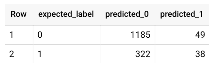
This table can be interpreted in the following way:

Make predictions using BigQuery ML
Once the ideal model was available, we ran ML.PREDICT to make predictions. For propensity modeling, the most important output is the probability of a behavior occurring. The following query returns the probability that the user will return after 24 hrs. The higher the probability and closer it is to 1, the more likely the user is predicted to return, and the closer it is to 0, the more likely the user is predicted to churn.
SELECTuser_pseudo_id,returned,predicted_returned,predicted_returned_probs[OFFSET(0)].prob as probability_returnedFROMML.PREDICT(MODEL bqmlga4.churn_logreg,(SELECT * FROM bqmlga4.train)) #can be replaced with a proper test dataset
Utilize predictions for activation
Once the model predictions are available for your users, you can activate this insight in different ways. In our analysis, we used user_pseudo_id as the user identifier. However, ideally, your app should send back the user_id from your app to Google Analytics. In addition to using first-party data for model predictions, this will also let you join back the predictions from the model into your own data.
- You can import the model predictions back into Google Analytics as a user attribute. This can be done using the Data Import feature for Google Analytics 4. Based on the prediction values you can Create and edit audiences and also do Audience targeting. For example, an audience can be users with prediction probability between 0.4 and 0.7, to represent users who are predicted to be “on the fence” between churning and returning.
- For Firebase Apps, you can use the Import segments feature. You can tailor user experience by targeting your identified users through Firebase services such as Remote Config, Cloud Messaging, and In-App Messaging. This will involve importing the segment data from BigQuery into Firebase. After that you can send notifications to the users, configure the app for them, or follow the user journeys across devices.
- Run targeted marketing campaigns via CRMs like Salesforce, e.g. send out reminder emails.
You can find all of the code used in this blogpost in the Github repository:
What’s next?
Continuous model evaluation and re-training
As you collect more data from your users, you may want to regularly evaluate your model on fresh data and re-train the model if you notice that the model quality is decaying.
Continuous evaluation—the process of ensuring a production machine learning model is still performing well on new data—is an essential part in any ML workflow. Performing continuous evaluation can help you catch model drift, a phenomenon that occurs when the data used to train your model no longer reflects the current environment.
To learn more about how to do continuous model evaluation and re-train models, you can read the blogpost: Continuous model evaluation with BigQuery ML, Stored Procedures, and Cloud Scheduler
More resources
If you’d like to learn more about any of the topics covered in this post, check out these resources:
- BigQuery export of Google Analytics data
- BigQuery ML quickstart
- Events automatically collected by Google Analytics 4
- Qwiklabs: Create ML models with BigQuery ML
Or learn more about how you can use BigQuery ML to easily build other machine learning solutions:
- How to build demand forecasting models with BigQuery ML
- How to build a recommendation system on e-commerce data using BigQuery ML
Let us know what you thought of this post, and if you have topics you’d like to see covered in the future! You can find us on Twitter at @polonglin and @_mkazi_.Thanks to reviewers: Abhishek Kashyap, Breen Baker, David Sabater Dinter.
How Kinguin Notched Up Shopping Experience with Google Recommendations AI

6438
Of your peers have already read this article.
3:00 Minutes
The most insightful time you'll spend today!
Over 2.14 billion people worldwide are expected to buy online this year, according to Statista. Online retail sales will account for 22% of all purchases by 2023. But in a competitive retail landscape, positive interactions can mean the difference between a sale and an abandoned shopping cart.
One of the leading global marketplaces – Kinguin.net is a haven for gamers. Their bustling ecommerce business conducts over 500,000 new transactions monthly. Users will encounter over 50,000 unique digital products, from video games, gift cards, in-game items to computer software and services. With over 10 million registered users, Kinguin improved their experience by helping users find items quickly and deliver service at scale.
Helping customers find what they want, fast
Because of Kinguin’s high volume of users—both buyers and sellers—and breadth of digital products, browsing and shopping can be challenging. “Customers shop online for choice and convenience, but it can sometimes be overwhelming. We want anyone who shops at Kinguin to find what they are looking for quickly and easily,” says Viktor Romaniuk Wanli, Kinguin CEO and Founder.
Today’s retailers know that creating personalized shopping experiences is crucial for establishing and maintaining customer loyalty. Kinguin discovered their users were getting a rather standard retail experience. They wondered how they could offer them a more tailored, personalized experience.
They knew product recommendations were a great way to personalize experiences because they help customers discover products that match their tastes and preferences. But it’s not that easy to recommend products. Various shifting factors make recommendations much more complex:
- Customer behavior. Understanding customers is tough. How do you recommend something to a cold start user who’s never been to your site before? What happens when their behavior changes?
- Omnichannel context. According to Harvard Business Review, 73% of all customers use many channels when they buy. What happens when they go from desktop to mobile or from social media shopping to a proprietary app?
- Product data challenges. How do you recommend new products within a large catalog of items? What if your product data has sparse labeling or unstructured metadata?
Data wasn’t a problem for Kinguin. They had data orders, history, wishlists, and could collect events based on their platform interactions. It was the machine learning model expertise they lacked. So rather than building their own solution, they determined it was more cost effective for them to find a reliable partner. It was also essential that the solution integrated easily with Kubernetes, which enabled their global network.
With these considerations in mind, they applied for the Google Recommendations AI beta program. Kinguin became the first gaming e-commerce platform in Europe to use Recommendations AI when it launched in 2020.
Pro gamer move: using a fully managed AI service
Google Recommendations AI uses algorithms to deliver highly personalized suggestions tailored to a customer’s preferences. Google Cloud based these algorithms on the same research that powers models by YouTube search and Google Shopping. Algorithms are always being tuned and adjusted to focus on individuals themselves—not just items.
Many shopping AIs rely on manually provisioning infrastructure and training machine learning models. Instead, Recommendations AI’s deep learning models use item and user metadata to gain insights. It processes Kinguin’s thousands of products at scale, iterating in real time. First, Kinguin pieces together a customer’s history and shopping journey. Then, using Recommendations AI, they can serve up personalized products—even for long-tail products and cold-start users.
By leveraging internal tools, Kinguin didn’t need to start implementation from scratch. After a few trial sessions with Google Cloud engineers, they got started right away. Due to the fast-paced nature of a marketplace—i.e., price changes, out-of-stock items—Kinguin needed their recommendations to be as close to real time as possible. They used internal event buses to stream events and their product catalog directly to the recommendations API.
Kinguin rolled out in high-traffic areas, including their home page, product page, and category pages. They analyzed heat maps and scroll maps to figure out where to test placements. They also experimented with different recommendation models such as “recently bought together” and “you may like.” Engineers also factored in where they were implementing the models. For example, the “others you might like” model would fit best on the homepage, while “frequently bought together” made sense at checkout.
Understanding how product recommendations influence financials is critical for demonstrating the impact of personalization. Using BigQuery, Kinguin could analyze different cost projection models. BigQuery helped them dig into specific financial data to understand their margins and revenue gains.
Playing to win: enhanced customer experience
Since adopting Recommendations AI, Kinguin has improved both customer experience and satisfaction. Search times have shortened by 20 seconds. Additionally, their average cart value has increased by 5 EUR. Conversion rates have quadrupled since the outset. Click-thru rates have doubled, increasing by 2.16 on product pages and 2.8 times on recommendations pages.
“Google Recommendations AI has helped us evolve our service, increase customer loyalty and satisfaction. It has also contributed to a significant rise in sales,” says Wanli. Kinguin is already thinking about other ways of enhancing user experiences with recommendations. Ideas include their checkout process, other landing pages, and email marketing.
Kinguin’s journey with Google Cloud shows how companies can leverage AI to optimize sales and deliver high-performing, low-latency recommendations to any customer touchpoint.
Learn more about Recommendations AI and Google Cloud AI and machine learning solutions.
How Google Cloud & NGIS’ Partnership Powers Sustainability & Responsible Sourcing for Consumer Brands

6194
Of your peers have already read this article.
2:00 Minutes
The most insightful time you'll spend today!
In the competitive world of consumer goods, sustainability matters more than ever. In recent Google survey, 82% of consumers said sustainability is more top of mind now than it was before COVID-191 and 78% said that big businesses have a role to play in helping to fight climate change.2 As well as delivering on customers’ heightened expectations, sustainable business practices can help organizations reduce waste and lower operational costs and even help attract top talent.
Not only is sustainability good for business performance and the bottom line, it’s great for the planet, too. And it’s something we care deeply about at Google. Since our earliest days, we have focused on developing services that significantly improve the lives of billions of people while operating our business in an environmentally sustainable way. In 2007, we were the first major company to become carbon neutral, and in 2017 we were the first to achieve 100% renewable energy. Today, we proudly operate the cleanest cloud in the industry. We’ve also been powering humanitarian, scientific, and environmental initiatives studying geospatial information and making it available for analysis via Google Earth Engine.
Powering the future of responsible sourcing
How does all this relate to CPG supply chains? The world relies on raw materials like palm oil, soy, and cocoa to produce the items we consume every day—such as coffee, chocolate, frozen foods, shampoo, toothpaste, cosmetics, and even household cleaning products. Yet as demand for these materials continues to grow, forests are under threat. Change is needed.
As sustainability moves further into the spotlight, in-demand crops face increased supplier scrutiny. Environmentally conscious companies want to know what percentage of their raw materials is sourced from deforestation-free suppliers—and how they can improve that number. Until recently, many CPG brands have found it hard to get real-time, reliable visibility into operations at a local supplier level, globally.
Google Cloud, in partnership with NGIS, is helping brands gain a deeper understanding of raw material sourcing practices across supplier networks, so they can improve supplier performance and compliance in the fight against deforestation. The TraceMark solution, developed by NGIS, uses Google Earth Engine and BigQuery to analyze and visualize how suppliers behave over time.
Google Earth Engine is the world’s largest archive of open Earth data. It combines a multi-petabyte catalog of satellite imagery and geospatial datasets with planetary-scale analysis capabilities to help people detect changes, map trends, and quantify differences on the Earth’s surface.With Earth Engine, organizations can analyze the potential social, and environmental impacts of the decision they make.
Together, TraceMark, Google Earth Engine and BigQuery help companies visualize, monitor, and measure the impact of suppliers’ farming practices. The process starts with Earth Engine, which aggregates and harmonizes planetary data into images that it has been collecting for decades. Then, boundary maps for different suppliers are created and NGIS applies climate data science and machine learning to turn pixels into insights. Finally, BigQuery and Vertex AI -Google Cloud’s unified artificial intelligence platform are used to produce supplier scoring, which is integrated into downstream ERP and procurement systems to support more informed decision-making.
These efforts support the responsible sourcing of raw materials by making supply chains more agile, transparent and traceable.
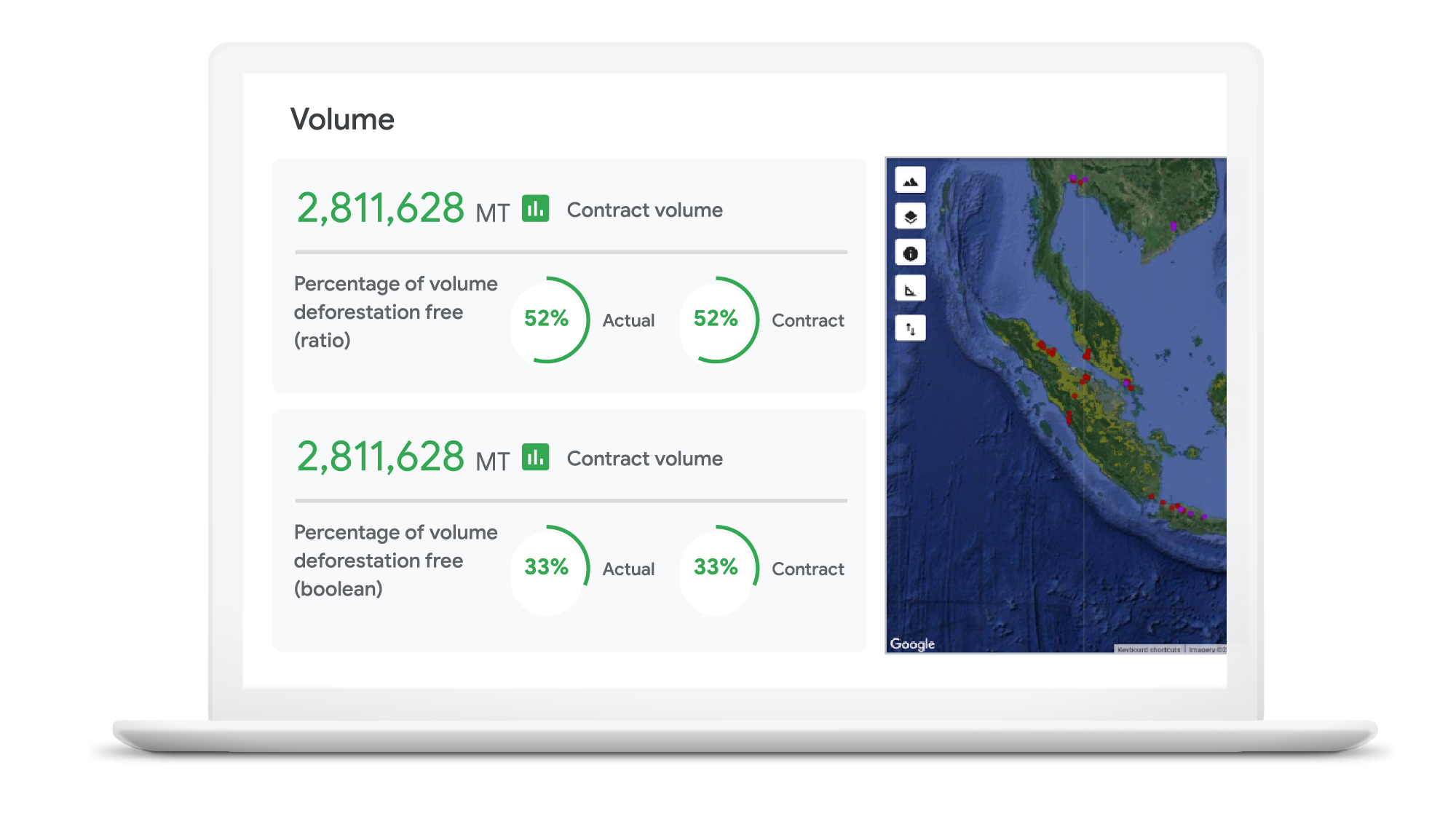
“NGIS is thrilled to work with Google Cloud and its partners to enable business accountability for sustainable practices at all levels of their supply chain,” said Nathan Eaton, Executive Director, NGIS. “Google Earth Engine provides unique geospatial capability that [gives] leaders visibility and control over their environmental footprint and that of their suppliers in a way that was not previously possible.”
Unilever commits to working towards a deforestation-free supply chain
Unilever is a great example of a company committed to using technology in the quest to become more sustainable. Since 2020, Unilever has partnered with Google Cloud to use data for eco-friendly decision-making, particularly when it comes to sustainable commodity sourcing.
By combining the power of cloud computing with satellite imagery and AI, we’re helping Unilever build a more holistic view of the forests, water cycles, and biodiversity that intersect its supply chain. By gaining a complete picture of these ecosystems, Unilever can detect deforestation while simultaneously prioritizing critical areas of forest and habitats in need of protection.
The cleanest cloud for your sustainable transformation
We are excited to bring Google Earth Engine and NGIS to our CPG customers to help them meet their sustainability goals. Looking ahead, we’re committed to furthering our own ambitious sustainability goals and empowering CPG brands with the technology to do more for our environment and our shared future.
Contact your cloud seller to learn more about Tracemark sustainable sourcing solutions and how Google Cloud can help you advance your sustainability initiatives.
Explore TraceMark on the Google Cloud Marketplace
To know more about how we are helping CPGs transform digitally read this ebook
1. Google/C Space, BR, FR, DE, IN, MX, U.K., U.S., qualitative survey activity, n = 528, Nov. 24–Nov. 26, 2020.
2. Google/Ipsos, Google Sustainability, BR, FR, DE, IN, JP, U.K., U.S., n=16,959 online population 18–70, July 2021.
5447
Of your peers have already watched this video.
1:30 Minutes
The most insightful time you'll spend today!
Skincare Firm Scales 4X in Minutes with SAP on Google Cloud
As the number one skincare brand in the United States, Rodan + Fields must support its team of over 300,000 of independent contractors as well as work to ensure a really personalized experience for customers. To keep pace with the company’s growth, Rodan + Fields realized it needed a more modern, scalable platform for its SAP environment.
After implementing both SAP ERP and SAP Hybris on Google Cloud, Rodan + Fields can focus on its business instead of infrastructure. It can scale four times its size in less than five minutes. Also, BigQuery is now used for data analysis to support critical business decisions.
With SAP on Google Cloud consultants can have 100% confidence that Rodan + Fields systems will provide them the insight, data and tools to succeed.
Google Cloud’s Transfer Services Helps Move Nuro’s Petabytes of Data from Edge to the Cloud

5147
Of your peers have already read this article.
3:00 Minutes
The most insightful time you'll spend today!
Engineers that build last-mile delivery services belong to an elite order, a hallowed subcategory. Delivery customers are incredibly demanding when it comes to speed and convenience, and the services they use must take variables like increased traffic, road conditions, human error, and even driver availability into account every day.
Nuro is a company with a new approach to delivery services. Nuro has a fleet of autonomous vehicles designed to address many of the problems related to last-mile delivery. And every day, these vehicles — and their sensors — generate a lot of data before parking for the night. For Nuro engineers, that data can help them understand the impact of new on-road features, make improvements to their vehicles’ software, and ensure even better deliveries for their customers.
For Nuro, the key challenge is how to move petabytes of data as quickly, securely, and easily as possible from their edge environments, like vehicle depots, to Google’s Cloud Storage. For this delivery effort, Nuro selected Google’s Transfer Appliance with its new online transfer capability, now generally available.
Helping Nuro to speed up data delivery from the edge to the cloud
Like many Google Cloud customers, Nuro collects data from remote environments, like vehicle depots, that have different networking and storage capabilities when compared to a traditional data center. For a transfer solution to be effective moving unstructured data from these environments to the cloud, the solution needs to be easy to deploy and automate, while still providing similar performance as a more complicated alternative.
The Transfer Appliance was built for this use case. It arrives to customers as a physical appliance with a preconfigured version of Google’s Storage Transfer Service software already installed. Customers can move files to the appliance by using SFTP or SCP, or, alternately, can mount the appliance as an NFS share and copy target. Data can be stored locally on the appliance or transferred over the network, and secure encryption — at-rest and in-flight — is enabled by default.
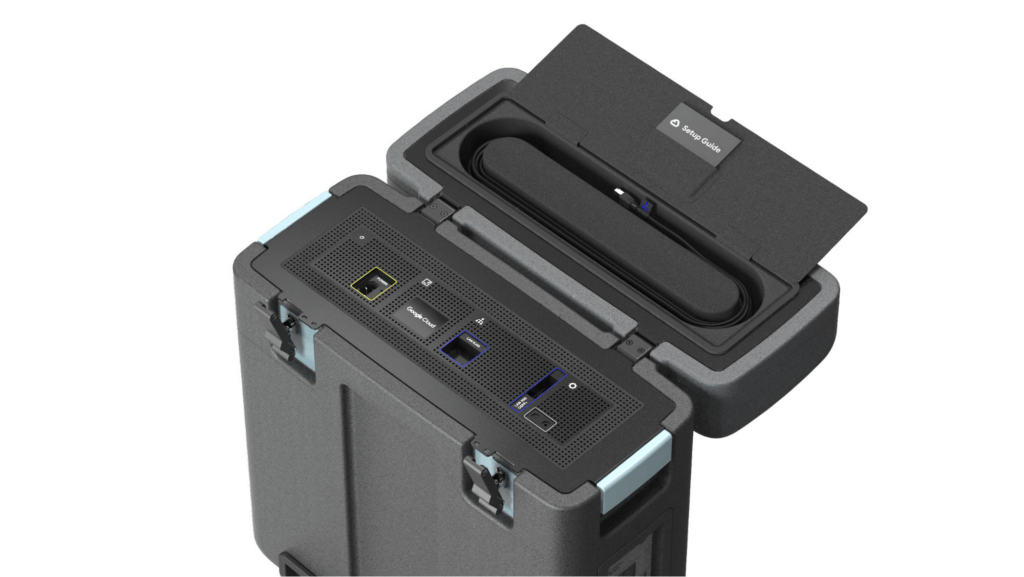
With these new appliances, Nuro will be able to automate much of their storage transfer needs. When their autonomous vehicles return to the depot, they can move data like software logs, LIDAR data, and sensor data — all ideal fits for Google’s Cloud Storage — from parked vehicles to the Transfer Appliance. Online transfers can then be performed throughout the day, ensuring a steady stream of valuable data in the cloud for developers to analyze and use in their nightly builds. All of this will help Nuro’s engineering leaders like Jie Pan to run more productive development teams with less operational overhead.
“Our autonomous vehicles generate a tremendous amount of useful data, and our goal is to get that data to our engineers as soon as possible,” said Jie Pan, Engineering Manager at Nuro. “When vehicles return to the depot, we can move data hourly into Cloud Storage over the network. We also have the flexibility to return the Transfer Appliance back to Google Cloud. Most importantly, this rapid transfer architecture gives a meaningful boost to engineering productivity and development velocity.”
Going the extra mile
Engineering and infrastructure leaders understand the value of delivering the right data to the right teams, as fast as possible. By adding preconfigured, over-the-network transfer into a turnkey Transfer Appliance, Google Cloud customers can more easily automate these data deliveries by scheduling regular migrations of on-premises files, objects, and other unstructured data to our Cloud Storage.
As Nuro continues to grow their manufacturing and testing footprint, they plan to use Transfer Appliances to further scale and simplify their data migration from on-premises to Google Cloud. Cutting the time to migrate their data by more than half will make for happier, more productive developers, and that will help Nuro bring us all the future of delivery a little faster.
If you’d like to learn more about Transfer Appliance and its new online transfer capability, click here or reach out to your Google Cloud account team.
More Relevant Stories for Your Company

Why Data Cloud Matters for Business Transformation
I’m so excited to be part of Google Cloud. Data has been a longstanding part of my career and it is at the heart of business transformation. Many companies have mastered the ability to collect data and have mechanisms in place to draw on some of it to solve business

Guide for Measuring Cloud Spanner Performance for Your Custom Workload
Database migration to a new database platform or technology can be daunting for various reasons. One of the common concerns is database performance. It is hard to evaluate database performance early in the evaluation cycle without performing actual data migration and application changes. This becomes even more important in the

Google Introduces BigQuery Connector for SAP to Power Customers’ Data Analytics Strategy
Google Cloud has a genuine passion for solving technology problems that make a difference for our customers. With the release of our BigQuery Connector for SAP, we're taking a another big step towards solving a major challenge for SAP customers with a quick, easy, and inexpensive way to integrate SAP data

Revolutionizing Healthcare Operations with Data Engine Accelerators
Healthcare leaders are increasingly challenged to drive operational improvements throughout their facilities, and inefficiencies can cost organizations both time and money and impact patient outcomes. Additionally, staffing shortages and employee burnout remain a major concern in healthcare. Addressing these challenges can help healthcare providers improve organizational operations, patient experiences and
