New Capabilities in BigQuery to Ease Anomalies Detection in the Absence of Labeled Data

Blog

New Capabilities in BigQuery to Ease Anomalies Detection in the Absence of Labeled Data

6321

Of your peers have already read this article.

4:00 Minutes

The most insightful time you'll spend today!

The new anomaly detection capabilities in BigQuery ML makes use of unsupervised machine learning to ease anomaly detection in the absence of labeled data. Read the blog to help your users work with time-series and non time series model.

When it comes to anomaly detection, one of the key challenges that many organizations face is that it can be difficult to know how to define what an anomaly is. How do you define and anticipate unusual network intrusions, manufacturing defects, or insurance fraud? If you have labeled data with known anomalies, then you can choose from a variety of supervised machine learning model types that are already supported in BigQuery ML. But what can you do if you don’t know what kind of anomaly to expect, and you don’t have labeled data? Unlike typical predictive techniques that leverage supervised learning, organizations may need to be able to detect anomalies in the absence of labeled data.

Today we are announcing the public preview of new anomaly detection capabilities in BigQuery ML that leverage unsupervised machine learning to help you detect anomalies without needing labeled data. Depending on whether or not the training data is time series, users can now detect anomalies in training data or on new input data using a new ML.DETECT_ANOMALIES function (documentation), with the following models:

Autoencoder model, now in Public Preview (documentation)
K-means model, already GA (documentation)
ARIMA_PLUS time series model, already GA (documentation)

How does anomaly detection with ML.DETECT_ANOMALIES work?

To detect anomalies in non-time-series data, you can use:

K-means clustering models: When you use ML.DETECT_ANOMALIES with a k-means model, anomalies are identified based on the value of each input data point’s normalized distance to its nearest cluster. If that distance exceeds a threshold determined by the contamination value provided by the user, the data point is identified as an anomaly.
Autoencoder models: When you use ML.DETECT_ANOMALIES with an autoencoder model, anomalies are identified based on the reconstruction error for each data point. If the error exceeds a threshold determined by the contamination value, it is identified as an anomaly.

To detect anomalies in time-series data, you can use:

ARIMA_PLUS time series models: When you use ML.DETECT_ANOMALIES with an ARIMA_PLUS model, anomalies are identified based on the confidence interval for that timestamp. If the probability that the data point at that timestamp occurs outside of the prediction interval exceeds a probability threshold provided by the user, the datapoint is identified as an anomaly.

Below we show code examples of anomaly detection in BigQuery ML for each of the above scenarios.

Anomaly detection with a k-means clustering model

You can now detect anomalies using k-means clustering models, by running ML.DETECT_ANOMALIES to detect anomalies in the training data or in new input data. Begin by creating a k-means clustering model:

Language: SQL

  CREATE MODEL `mydataset.my_kmeans_model`
OPTIONS(
  MODEL_TYPE = 'kmeans',
  NUM_CLUSTERS = 8,
  KMEANS_INIT_METHOD = 'kmeans++'
) AS
SELECT 
  * EXCEPT(Time, Class) 
FROM 
  `bigquery-public-data.ml_datasets.ulb_fraud_detection`;

With the k-means clustering model trained, you can now run ML.DETECT_ANOMALIES to detect anomalies in the training data or in new input data.
To detect anomalies in the training data, use ML.DETECT_ANOMALIES with the same data used during training:

Language: SQL

  SELECT
  *
FROM
  ML.DETECT_ANOMALIES(MODEL `mydataset.my_kmeans_model`,
                      STRUCT(0.02 AS contamination),
                      TABLE `bigquery-public-data.ml_datasets.ulb_fraud_detection`);

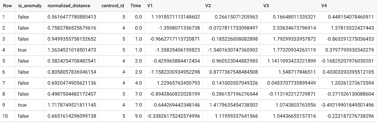
To detect anomalies in new data, use ML.DETECT_ANOMALIES and provide new data as input:

Language: SQL

  SELECT
  *
FROM
  ML.DETECT_ANOMALIES(MODEL `mydataset.my_kmeans_model`,
                      STRUCT(0.02 AS contamination),
                      (SELECT * FROM `mydataset.newdata`));

How does anomaly detection work for k-means clustering models?

Anomalies are identified based on the value of each input data point’s normalized distance to its nearest cluster, which, if exceeds a threshold determined by the contamination value, is identified as an anomaly. How does this work exactly? With a k-means model and data as inputs, ML.DETECT_ANOMALIES first computes the absolute distance for each input data point to all cluster centroids in the model, then normalizes each distance by the respective cluster radius (which is defined as the standard deviation of the absolute distances of all points in this cluster to the centroid). For each data point, ML.DETECT_ANOMALIES returns the nearest centroid_id based on normalized_distance, as seen in the screenshot above. The contamination value, specified by the user, determines the threshold of whether a data point is considered an anomaly. For example, a contamination value of 0.1 means that the top 10% of descending normalized distance from the training data will be used as the cut-off threshold. If the normalized distance for a datapoint exceeds the threshold, then it is identified as an anomaly. Setting an appropriate contamination will be highly dependent on the requirements of the user or business.

For more information on anomaly detection with k-means clustering, please see the documentation here.

Anomaly detection with an autoencoder model

You can now detect anomalies using autoencoder models, by running ML.DETECT_ANOMALIES to detect anomalies in the training data or in new input data.

Begin by creating an autoencoder model:

Language: SQL

  CREATE MODEL `mydataset.my_autoencoder_model`
OPTIONS(
  model_type='autoencoder',
  activation_fn='relu',
  batch_size=8,
  dropout=0.2,  
  hidden_units=[32, 16, 4, 16, 32],
  learn_rate=0.001,
  l1_reg_activation=0.0001,
  max_iterations=10,
  optimizer='adam'
) AS 
SELECT 
  * EXCEPT(Time, Class) 
FROM 
  `bigquery-public-data.ml_datasets.ulb_fraud_detection`;

To detect anomalies in the training data, use ML.DETECT_ANOMALIES with the same data used during training:

Language: SQL

  SELECT
  *
FROM
  ML.DETECT_ANOMALIES(MODEL `mydataset.my_autoencoder_model`,
                      STRUCT(0.02 AS contamination),
                      TABLE `bigquery-public-data.ml_datasets.ulb_fraud_detection`);

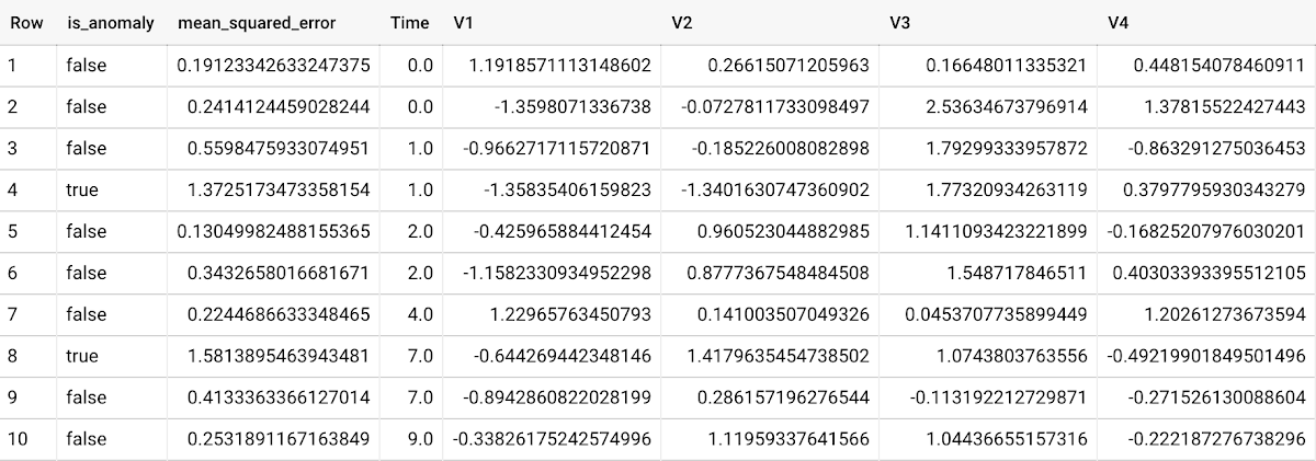
To detect anomalies in new data, use ML.DETECT_ANOMALIES and provide new data as input:

Language: SQL

  SELECT
  *
FROM
  ML.DETECT_ANOMALIES(MODEL `mydataset.my_autoencoder_model`,
                      STRUCT(0.02 AS contamination),
                      (SELECT * FROM `mydataset.newdata`));

How does anomaly detection work for autoencoder models?

Anomalies are identified based on the value of each input data point’s reconstructed error, which, if exceeds a threshold determined by the contamination value, is identified as an anomaly. How does this work exactly? With an autoencoder model and data as inputs, ML.DETECT_ANOMALIES first computes the mean_squared_error for each data point between its original values and its reconstructed values. The contamination value, specified by the user, determines the threshold of whether a data point is considered an anomaly. For example, a contamination value of 0.1 means that the top 10% of descending error from the training data will be used as the cut-off threshold. Setting an appropriate contamination will be highly dependent on the requirements of the user or business.

For more information on anomaly detection with autoencoder models, please see the documentation here.

Anomaly detection with an ARIMA_PLUS time-series model

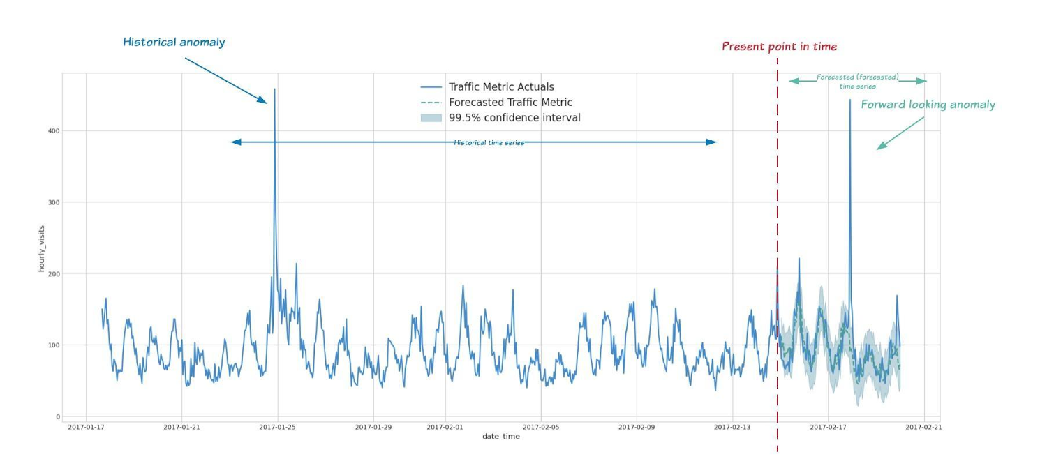
With ML.DETECT_ANOMALIES, you can now detect anomalies using ARIMA_PLUS time series models in the (historical) training data or in new input data. Here are some examples of when might you want to detect anomalies with time-series data:

Detecting anomalies in historical data:

Cleaning up data for forecasting and modeling purposes, e.g. preprocessing historical time series before using them to train an ML model.
When you have a large number of retail demand time series (thousands of products across hundreds of stores or zip codes), you may want to quickly identify which stores and product categories had anomalous sales patterns, and then perform a deeper analysis of why that was the case.

Forward looking anomaly detection:

Detecting consumer behavior and pricing anomalies as early as possible: e.g. if traffic to a specific product page suddenly and unexpectedly spikes, it might be because of an error in the pricing process that leads to an unusually low price.
When you have a large number of retail demand time series (thousands of products across hundreds of stores or zip codes), you would like to identify which stores and product categories had anomalous sales patterns based on your forecasts, so you can quickly respond to any unexpected spikes or dips.

How do you detect anomalies using ARIMA_PLUS? Begin by creating an ARIMA_PLUS time series model:

Language: SQL

  CREATE OR REPLACE MODEL mydataset.my_arima_plus_model
OPTIONS(
  MODEL_TYPE='ARIMA_PLUS',
  TIME_SERIES_TIMESTAMP_COL='date',
  TIME_SERIES_DATA_COL='total_amount_sold',
  TIME_SERIES_ID_COL='item_name',
  HOLIDAY_REGION='US' 
) AS
SELECT
  date,
  item_description AS item_name,
  SUM(bottles_sold) AS total_amount_sold
FROM
  `bigquery-public-data.iowa_liquor_sales.sales`
GROUP BY
  date,
  item_name
HAVING
  date BETWEEN DATE('2016-01-04') AND DATE('2017-06-01')
  AND item_name IN ("Black Velvet", "Captain Morgan Spiced Rum",
    "Hawkeye Vodka", "Five O'Clock Vodka", "Fireball Cinnamon Whiskey");

To detect anomalies in the training data, use ML.DETECT_ANOMALIES with the model obtained above:

Language: SQL

  SELECT
  *
FROM
  ML.DETECT_ANOMALIES(MODEL `mydataset.my_arima_plus_model`,
                      STRUCT(0.8 AS anomaly_prob_threshold));

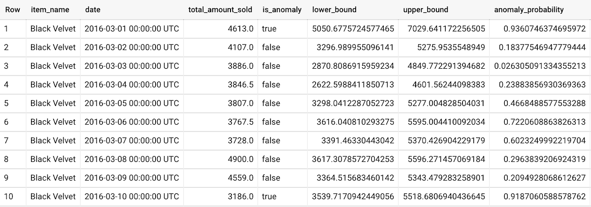
To detect anomalies in new data, use ML.DETECT_ANOMALIES and provide new data as input:

Language: SQL

  WITH
  new_data AS (
  SELECT
    date,
    item_description AS item_name,
    SUM(bottles_sold) AS total_amount_sold
  FROM
    `bigquery-public-data.iowa_liquor_sales.sales`
  GROUP BY
    date,
    item_name
  HAVING
    date BETWEEN DATE('2017-06-02')
    AND DATE('2017-10-01')
    AND item_name IN ('Black Velvet',
      'Captain Morgan Spiced Rum',
      'Hawkeye Vodka',
      "Five O'Clock Vodka",
      'Fireball Cinnamon Whiskey') )
SELECT
  *
FROM
  ML.DETECT_ANOMALIES(MODEL `mydataset.my_arima_plus_model`,
    STRUCT(0.8 AS anomaly_prob_threshold),
    (SELECT
      *
    FROM
      new_data));

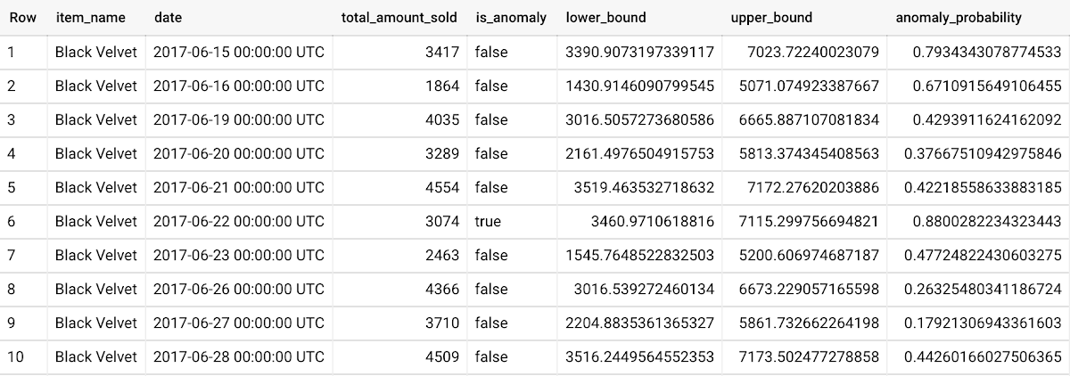
For more information on anomaly detection with ARIMA_PLUS time series models, please see the documentation here.

Thanks to the BigQuery ML team, especially Abhinav Khushraj, Abhishek Kashyap, Amir Hormati, Jerry Ye, Xi Cheng, Skander Hannachi, Steve Walker, and Stephanie Wang.

6504

Of your peers have already watched this video.

46:30 Minutes

The most insightful time you'll spend today!

Case Study

The Inside Story of How Home Depot Migrated to Google BigQuery From an On-prem DW Solution

In the media, you will often hear story of how born-in-the-cloud companies manage with massive infrastructure.

But it is one thing is to be a startup, and build infrastructure with bespoke requirements. And quite another to have a complex, multinational organization with online, with mobile, with brick-and-mortar presence, and hundreds of thousands of SKUs and professional services, and many, many years of technology, innovation, and really smart engineers.

This is the second story. The story of how The Home Depot, the number-one home improvement retailer in the US pulled of that feat.

The Home Depot has over 2,200 stores, over 4 lakh associates, and 2017 revenues of over a $100 billion.

In this video, Rick Ramaker, technology director, data analytics at The Home Depot, and Kevin Scholz, distinguished engineer, The Home Depot, talk about how the company transformed and modernised its data warehousing, the challenges they faced and the benefits they accrued from the project.

It’s a fascinating watch!

Blog

Over 700 SaaS Companies Trust Google’s Data Cloud to Build Intelligent Apps!

3490

Of your peers have already read this article.

5:00 Minutes

The most insightful time you'll spend today!

Data monetization is a compelling proposition for SaaS companies to diversify revenue streams and make most of their customer data. Google's data cloud is the heart of 700 tech companies to power their apps using data and ML products. Learn more!

Today, a typical enterprise uses over 100 SaaS applications while large organizations commonly use over 400 apps. These applications contain valuable data on customers, suppliers, employees, products and more, offering the potential for valuable insights and powerful workflows. However, in the past, this data has often remained siloed and underutilized, even within an application.

Customer demand is driving an unprecedented wave of innovation across the SaaS industry, with providers building intelligence into their applications through rich analytical and AI/ML capabilities, and enabling their customers’ data ecosystems through real time data sharing. The data cloud platform powering these applications is a critical factor in companies’ ability to innovate and optimize efficiency, while keeping its customer’s data secure.

Today, over 700 tech companies including Zoominfo, Equifax, Exabeam, Bloomreach, and Quantum Metric power their products and businesses using Google’s data cloud. This week at the Data Cloud Summit, we announced the Built with BigQuery initiative which helps ISVs get started building applications using data and machine learning products. By providing dedicated access to technology, expertise and go to market programs, this initiative allows tech companies to accelerate, optimize and amplify their success.

“Enabling customers to gain superior insights and intelligence from data is core to the ZoomInfo strategy,” ZoomInfo CEO Henry Schuck says. “We are excited about the innovation Google Cloud is bringing to market and how it is creating a differentiated ecosystem that allows customers to gain insights from their data securely, at scale, and without having to move data around. Working with the Built with BigQuery initiative team enables us to rapidly gain deep insight into the opportunities available and accelerate our speed to market.”

Building intelligent SaaS applications with a unified data platform

Google’s data cloud provides a complete platform for building data-driven applications, from simplified data ingestion, processing and storage to powerful analytics, AI/ML and data sharing capabilities, all seamlessly integrated with Google Cloud’s open, secure, sustainable platform. With a huge partner ecosystem and support for multicloud, open source tools and APIs, we provide technology companies the portability and extensibility they need to avoid data lock-in.

Through the Built with BigQuery initiative, we are helping tech companies to build the next-gen SaaS applications on Google’s data cloud with simplified access to technology, dedicated engineering support and joint go to market programs.

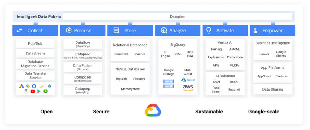
Exabeam, a next generation cybersecurity solution, is a great example. The company leverages Google’s data cloud to provide their customers with a “limitless-scale” cybersecurity solution.

“Built with Google’s data cloud, Exabeam’s limitless-scale cybersecurity platform helps enterprises respond to security threats faster and more accurately” said Sanjay Chaudhary, VP of Products at Exabeam. “We are able to ingest data from over 500 security vendors, convert unstructured data into security events, and create a common platform to store them in a cost effective way. The scale and power of Google’s data cloud enables our customers to search multi-year data and detect threats in seconds.”

Foster innovation and unlock new business models through data sharing

Data becomes even more valuable when shared. According to research, the global data monetization market size is growing at a CAGR of 47.9% and is projected to reach $11.7 Billion by 2026. It’s a compelling proposition for SaaS companies as it enables them to deliver increased value for their customers while expanding their own partner ecosystem, increasing stickiness and unlocking new revenue streams.

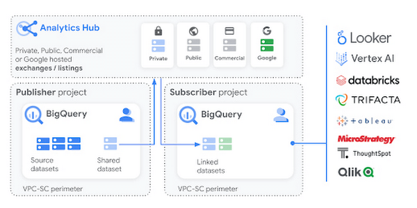
Google Cloud’s strategy for data sharing encompasses three key areas: secure data sharing in BigQuery, the ability to create private and public exchanges alongside commercial and public datasets in Analytics Hub, and a robust ecosystem of premier partner and Google data.

Through the real-time data sharing capabilities of BigQuery, SaaS companies are enabling their customers to combine their data with the customer’s own proprietary data, and other third-party data sources, to derive 360-degree insights. Over 4,500 organizations share more than 250 Petabytes of data weekly in BigQuery, not accounting for intra-organizational data sharing*.

For example, manufacturers can get real-time visibility into their entire supply chain by combining datasets from ISVs, such as supply chain innovator, Blume Global, and data publishers.

“Our partnership with Google Cloud is helping us achieve our mission to build the next-generation supply chain operating system. Blume Maps, our digital twin of the supply chain world built with Google’s data cloud, allows our customers to generate accurate lead times, real-time shipment location and ETAs” said Blume Global CEO Pervinder Johar. “We apply the power of Google Cloud’s data and analytics capabilities to our growing database of over 1.5 million global data points to feed our lead time and dynamic ETA engine. We are also able to create data twins of unique logistics data and share with users around the globe.”

Google Cloud’s Analytics Hub is a fully-managed service built on BigQuery that allows organizations to efficiently and securely exchange valuable data and analytics assets across any organizational boundary. With unique datasets that are always-synchronized and bi-directional sharing, you can create a rich and trusted data ecosystem between business units or partnerships–one in which everyone gains value immediately.

“As external data becomes more critical to organizations across industries, the need for a unified experience between data integration and analytics has never been more important. We are proud to be working with Google Cloud to power the launch of Analytics Hub, feeding hundreds of pre-engineered data pipelines from hundreds of external datasets,” said Dan Lynn, SVP Product at Crux. “The sharing capabilities that Analytics Hub delivers will significantly enhance the data mobility requirements of practitioners, and the Crux data integration platform stands ready to quickly integrate any external data source and deliver on behalf of Google Cloud and its clients.”

Innovate, optimize and amplify with Google Cloud

The Built with BigQuery initiative provides access to technology, expertise and go-to-market:.

Access to Technology: Get started fast with a Google-funded, pre-configured sandbox. Access Cloud Credits to fund your, and your customer’s, POCs and apply for innovative pricing models designed for ISVs.
Access to Expertise: Accelerate and optimize product design and architecture with access to designated experts in building data-driven SaaS applications from the ISV Center of Excellence, providing insight into key use cases, architectural patterns and best practices. Access experts from across Google to enable co-innovation with products such as Earth Engine and Google Marketing Platform.
Access to Go-to-market: Amplify your success with joint marketing programs to drive awareness, generate demand and increase adoption.

Get Started

Start building your applications on Google Cloud with $300 in free credits or apply for the Built with BigQuery initiative.

*As of November, 2021, within a typical 7 day period in BigQuery, and not accounting for intra-organizational data sharing.

Blog

Optimizing Terabyte-scale PostgreSQL Migrations to Cloud SQL Using Searce

3025

Of your peers have already read this article.

2:30 Minutes

The most insightful time you'll spend today!

In this blog, we share with you how Searce reduced downtime by 98% while migrating terabyte-scale PostgreSQL database to Cloud SQL using the Database Migration Service.

Google Cloud allows you to move your PostgreSQL databases to Cloud SQL with Database Migration Service (DMS). DMS gives you the ability to replicate data continuously to the destination database, while the source is live in production, enabling you to migrate with minimum downtime.

However, terabyte-scale migrations can be complex. For instance, if your PostgreSQL database has Large Objects, then you will require some downtime to migrate them manually as that is a limitation of DMS. There are few more such limitations – check out known limitations of DMS. If not handled carefully, these steps can extend the downtime during cutover, lead to performance impact on the source instance, or even delay the project delivery date. All this may mean significant business impact.

Searce is a technology consulting company, specializing in modernizing application and database infrastructure by leveraging cloud, data and AI. We empower our clients to accelerate towards the future of their business. In our journey, we have helped dozens of clients migrate to Cloud SQL, and have found terabyte-scale migrations to be the toughest for the reasons mentioned earlier.

This blog centers around our work in supporting an enterprise client whose objective was to migrate dozens of terabyte scale, mission-critical PostgreSQL databases to Cloud SQL with minimum downtime. Their largest database was 20TB in size and all the databases had tables with large objects and some tables did not have primary keys. Note that DMS had a limitation of not supporting migration of tables without a primary key during the time of this project. In June 2022, DMS released an enhancement to support the migration of tables without a primary key.

In this blog, we share with you our learnings about how we simplified and optimized this migration, so that you can incorporate our best practices into your own migrations. We explore mechanisms to reduce the downtime required for operations not handled by DMS by ~98% with the use of automation scripts. We also explore database flags in PostgreSQL to optimize DMS performance and minimize the overall migration time by ~15%.

Optimize DMS performance with database flags

Once the customer made the decision to migrate PostgreSQL databases to Google Cloud SQL, we considered two key factors that would decide business impact – migration effort and migration time. To minimize effort for the migration of PostgreSQL databases, we leveraged Google Cloud’s DMS (Database Migration Service) as it is very easy to use and it does the heavy lifting by continuously replicating data from the source database to the destination Cloud SQL instance, while the source database is live in production.

How about migration time? For a terabyte-scale database, depending on the database structure, migration time can be considerably longer. Historically, we observed that DMS took around 3 hours to migrate a 1 TB database. In other cases, where the customer database structure was more complex, migration took longer. Thankfully, DMS takes care of this replication while the source database is live in production, so no downtime is required during this time. Nevertheless, our client would have to bear the cost of both the source and destination databases which for large databases, might be substantial. Meanwhile, if the database size increased, then replication could take even longer, increasing the risk of missing the customer’s maintenance window for the downtime incurred during cutover operations. Since the customer’s maintenance window was monthly, we would have to wait for 30 more days for the next maintenance window, requiring the customer to bear the cost of both the databases for another 30 days. Furthermore, from a risk management standpoint, the longer the migration timeframe, the greater the risk that something could go wrong. Hence, we started exploring options to reduce the migration time. Even the slightest reduction in migration time could significantly reduce the cost and risk.

We explored options around tuning PostgreSQL’s database flags on the source database. While DMS has its own set of prerequisite flags for the source instance and database, we also found that flags like shared_buffers, wal_buffers and maintenance_work_mem helped accelerate the replication process through DMS. These flags needed to be set to a specific value to get the maximum benefit out of each of them. Once set, their cumulative impact was a reduction in time for DMS to replicate a 1 TB database by 4 hours, that is, reduction of 3.5 days for a 20 TB database. Let’s dive into each of them.

Shared Buffers

PostgreSQL uses two buffers – its own internal buffer and the kernel buffered IO. In other words, that data is stored in memory twice. The internal buffer is called shared_buffers, and it determines the amount of memory used by the database for the operating system cache. By default this value is set conservatively low. However, increasing this value on the source database to fit our use case helped increase the performance of read heavy operations, which is exactly what DMS does once a job has been initialized.

After multiple iterations, we found that if the value was set to 55% of the database instance RAM, it boosted the replication performance (a read heavy operation) by a considerable amount and in turn reduced the time required to replicate the data.

WAL Buffers

PostgreSQL relies on Write-Ahead Logging (WAL) to ensure data integrity. WAL records are written to buffers and then flushed to disk. The flag wal_buffers, determines the amount of shared memory used for WAL data that has not yet been written to disk – records that are yet to be flushed. We found that increasing the value for wal_buffers from the default value of 16MB to about 3% of the database instance’s RAM significantly improved the write performance by writing fewer but larger files to the disk at each transaction commit.

Maintenance Work Mem

PostgreSQL maintenance operations, such as VACUUM, CREATE INDEX, and ALTER TABLE ADD FOREIGN KEY, consume their own specific memory. This memory is referred to as maintenance_work_mem. Unlike other operations, PostgreSQL maintenance operations can only be performed sequentially by the database. Setting a value significantly higher than the default value of 64 MB meant that no maintenance operation would block the DMS job. We found that maintenance_work_mem worked best at the value of 1 GB.

Resize source instance to avoid performance impact

Each of these three flags tune how PostgreSQL utilizes memory resources. Hence, it was imperative that before setting these flags, we needed to upsize the source database instance to accommodate them. Without upsizing the database instances, we could have caused application performance degradation, as more than half of the total database memory would be allocated to the processes managed by these flags.

We calculated the memory required by the flags mentioned above, and found that each flag needed to be set to a specific percentage of the source instance’s memory, irrespective of the existing values that might be set for the flags:

shared_buffers: 55% of source instance’s memory
wal_buffers: 3% of source instance’s memory
maintenance_work_mem: 1 GB

We added the individual memory requirements by the flags, and found that 58% of the RAM at least will be taken up by these memory flags. For example, if a source instance used 100GB of memory, 58GB would be taken up by shared_buffers and wal_buffers, and an additional 1GB by maintenance_work_mem. As the original value of these flags was very low (~200MB), we upsized the RAM of the source database instance by 60% in order to ensure that the migration did not impact source performance on the application live in production.

Avoid connection error with WAL sender timeout flag

While using Google Cloud’s DMS, if the connection is terminated between DMS and the Cloud SQL instance during the ‘Full Dump in Progress’ phase of the DMS job, the DMS job fails and needs to be reinitiated. Encountering timeouts, especially while migrating a terabyte-scale database, would mean multiple days’ worth of migration being lost and a delay in the cutover plan. For example, if the connection of the DMS job for a 20TB database migration is lost after 10 days, the DMS job will have to be restarted from the beginning, leading to 10 days’ worth of migration effort being lost.

Adjusting the WAL sender timeout flag (wal_sender_timeout) helped us avoid terminating replication connections that were inactive for a long time during the full dump phase. The default value for this flag is 60 seconds. To avoid these connections from terminating, and to avoid such high impact failures, we set the value of this flag to 0 for the duration of database migration. This would avoid connections getting terminated and allowed for smoother replication through the DMS jobs.

Generally, for all the database flags we talked about here, we advised our customer to restore the default flag values once the migration completed.

Reduce downtime required for DMS limitations by automation

While DMS does the majority of database migration through continuous replication when the source database instance is live in production, DMS has certain migration limitations that cannot be addressed when the database is live. For PostgreSQL, the known limitations of DMS include:

Any new tables created on the source PostgreSQL database after the DMS job has been initialized are not replicated to the destination PostgreSQL database.
Tables without primary keys on the source PostgreSQL database are not migrated. For those tables, DMS migrated only the schema. This is no longer a limitation after the June 2022 product update.
The large object (LOB) data type is not supported by DMS.
Only the schema for Materialized Views is migrated; the data is not migrated.
All data migrated is created under the ownership of cloudsqlexternalsync.

We had to address these aspects of the database migration manually. Since our client’s database had data with the large object data type, tables without primary keys, and frequently changing table structures that cannot be migrated by DMS, we had to manually export and import that data after DMS did most of the rest of the data migration. This part of database migration required downtime to avoid data loss. For a terabyte-scale database, this data can be in the hundreds of GBs, which means higher migration time and hence higher downtime. Furthermore, when you have dozens of databases to migrate, it can be stressful and error-prone for a human to perform these operations while on the clock during the cutover window!

This is where automation helped save the day! Automating the migration operations during the downtime period not only reduced the manual effort and error risk, but also provided a scalable solution that could be leveraged for the migration of 100s of PostgreSQL database instances to Cloud SQL. Furthermore, by leveraging multiprocessing and multithreading, we were able to reduce the total migration downtime for 100s of GBs of data by 98%, thereby reducing the business impact for our client.

How do we get there?

We laid out all the steps that need to be executed during the downtime – that is, after the DMS job has completed its replication from source to destination and before cutting over the application to the migrated database. You can see a chart mapping out the sequence of operations that are performed during the downtime period in Fig 1.

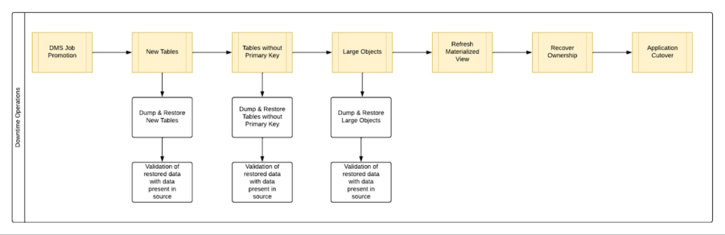
Fig 1: Downtime Migration – Sequential Approach

By automating all the downtime operations in this sequential approach, we observed that it took 13 hours for the entire downtime flow to execute for a 1 TB database. This included the migration of 250 MB in new tables, 60 GB in tables without primary keys and 150 GB in large objects.

One key observation we made was that, out of all the steps, only three steps took most of the time: migrating new tables, migrating tables without primary keys, and migrating large objects. These took the longest time because they all required dump and restore operations for their respective tables. However, these three steps did not have a hard dependency on each other as they individually targeted different tables. So we tried to run them in parallel as you can see in Fig 2. But the steps following them – ‘Refresh Materialized View’ and ‘Recover Ownership’ – had to be performed sequentially as they targeted the entire database.

However, running these three steps in parallel required upsizing the Cloud SQL instances, as we wanted to have sufficient resources available for each step. This led us to increase the Cloud SQL instances’ vCPU by 50% and memory by 40%, since the export and import operations depended heavily on vCPU consumption as opposed to memory consumption.

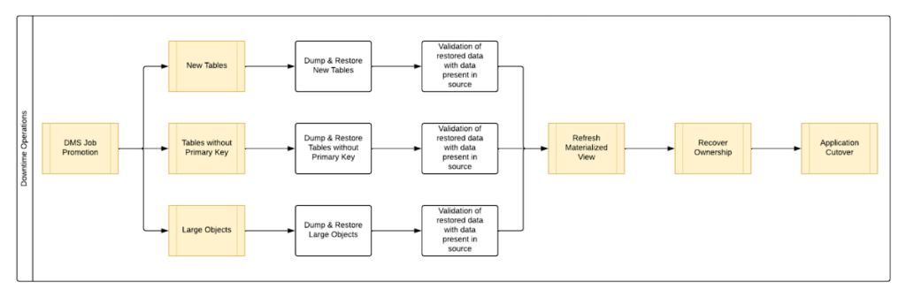
Fig 2: Downtime Migrations – Hybrid Approach

Migrating the new tables (created after the DMS job was initiated) and tables without primary keys was straightforward as we were able to leverage the native utilities offered by PostgreSQL – pg_dump and pg_restore. Both utilities process tables in parallel by using multiple threads– the higher the table count, the higher the number of threads that could be executed in parallel, allowing faster migration. With this revised approach, for the same 1 TB database, it still took 12.5 hours for the entire downtime flow to execute.

This improvement reduced the cutover downtime, but we still found that we needed a 12.5 hour window to complete all the steps. We then discovered that 99% of the time of downtime was taken up by just one step: exporting and importing 150 GB of large objects. It turned out that multiple threads could not be used to accelerate the dump and restore large objects in PostgreSQL. Hence, migrating the large objects single handedly extended the downtime for migration by hours. Fortunately, we were able to come up with a workaround for that.

Optimize migration of Large Object from PostgreSQL database

PostgreSQL contains a large objects facility that provides stream-style access to data stored in a special large-object structure. When large objects are stored, they are broken down into multiple chunks and stored in different rows of the database, but are connected under a single Object Identifier (OID). This OID can thus be used to access any stored Large Object. Although users can add large objects to any table in the database, under the hood, PostgreSQL physically stores all large objects within a database in a single table called pg_largeobjects.

While leveraging pg_dump and pg_restore for export and import of large objects, this single table – pg_largeobject, becomes a bottleneck as the PostgreSQL utilities cannot execute multiple threads for parallel processing, since it’s just one table. Typically, the order of operations for these utilities looks something like this:

pg_dump reads the data to be exported from the source database
pg_dump writes that data into the memory of the client where pg_dump is being executed
pg_dump writes from memory to the disk of the the client (a second write operation)
pg_restore reads the data from the client’s disk
pg_restore writes the data to the destination database

Normally, these utilities would need to be executed sequentially to avoid data loss or data corruption due to conflicting processes. This leads to further increase in migration time for large objects.

Our workaround for this single-threaded process involved two elements. First, with our solution, we eliminated the second write operation – write from memory to disk (point #3). Instead, once the data was read and written into memory, our program would begin the import process and write data to the destination database. Second, since pg_dump and pg_restore could not use multiple threads to process the large objects in just the pg_largeobjects table, we took it upon ourselves to develop a solution that could use multiple threads. The thread count was based on the number of OIDs in the table – pg_largeobjects, and break that single table into smaller chunks for parallel execution.

This approach brought down Large Object migration operation from hours to minutes, therefore bringing down the downtime needed for all operations to be completed that DMS cannot handle, for the same 1 TB database, from 13 hours to just 18 minutes. A reduction of ~98% in the required downtime.

Conclusion

After multiple optimizations and dry runs, we were able to develop a procedure for our client to migrate dozens of terabyte-scale PostgreSQL databases to Google Cloud SQL with a minimal business impact. We developed practices to optimize DMS-based migration by 15% using database flags and reduce downtime by 98% with the help of automation and innovation. These practices can be leveraged for any terabyte-scale migration of PostgreSQL databases to Google Cloud SQL to accelerate migration, minimize downtime and avoid performance impact on mission critical applications.

4227

Of your peers have already watched this video.

54:00 Minutes

The most insightful time you'll spend today!

Case Study

Behind the Scenes: How eBay Provides its Customers New Shopping Experiences

“If it exists in the world, you are likely to find it on eBay.” So they say. With 180 million buyers and a global presence in over 190 markets, it’s probably true. A company that emerged out of the ashes of the dot-com bubble, eBay today is one of the most renowned organizations in the world.

eBay catalog has over 1 billion listings available worldwide at any given point in time and over 15 million listings are added on a daily basis. That essentially means many datasets from different sources. And that was a challenge.

The company needed a scalable and flexible platform to efficiently enable new shopping experiences globally, showcasing unique eBay inventory. It needed to iterate quickly and integrate data-heavy AI technologies.

eBay turned to Cloud Bigtable from Google. Today, Cloud Bigtable handles eBay’s global catalog with billions of listings, scaling to hundreds of terabytes with many millions of reads and writes, and gigabytes of data transferred in and out every second.

This helped eBay synchronize its entire catalog over GCP in near real-time with low latency and high consistency. It also enabled the company to serve catalog data to other services on GCP with high read volume and low latency and keep and serve all listing images in GCP along with AI vision signatures.

Find out how.

Research Reports

Takeaways from Forrester’s Cloud Data Warehouse Q1 2021 Report

DOWNLOAD RESEARCH REPORTS

5130

Of your peers have already downloaded this article

20:00 Minutes

The most insightful time you'll spend today!

Cloud data warehouse (CDW) solutions have transformed the delivery of modern analytics and are known to have the capabilities to provision data warehouse of any size in a matter of minutes, autotune queries, scale resources including compute and storage on demand and auto-upgrade to the latest version. As the need for integrated, real-time and self-service analytics scale, CDW vendors continue to focus on native integration with data lakes and object stores; self-service to simplify access and administration for larger and more complex warehouses; and advanced capabilities on parallel processing, compression, partitioning, indexing, query optimization, and dynamic resource provisioning. The most common CDW use cases include customer analytics, AI/machine learning (ML)-based analytics, vertical-specific analytics, and real-time analytics. Customers that are looking to select a CDW vendor need to consider couple of factors.

Download the report learn more 13 leading CDW providers in the Forrester Wave: Cloud Data Warehouse, Q1 2021 report and also explore Google Cloud’s BigQuery for data warehousing.

How Kinguin Notched Up Shopping Experience with Google Recommendations AI

Over 2.14 billion people worldwide are expected to buy online this year, according to Statista. Online retail sales will account for 22% of all purchases by 2023. But in a competitive retail landscape, positive interactions can mean the difference between a sale and an abandoned shopping cart. One of the leading global

If your organization is one of the 52% of SAP customers whose top analytics pain point is data integration1, Google Cloud has got you covered.

How-to

Migrating From Oracle OLTP System to Cloud Spanner

Spanner uses certain concepts differently from other enterprise database management tools, so you might need to adjust your application to take full advantage of its capabilities. You might also need to supplement Spanner with other services from Google Cloud to meet your needs. Migration constraints When you migrate your application

“With Cloud Bigtable clusters in Asia, Europe, and the United States, we’re able to get low-latency data access all over the world, enabling Spotify to provide a seamless experience for our users.” Niklas Gustavsson, Chief Architect, Spotify

Webinar

Unlocking Data Value: Latest Data Platforms and Announcements at the Next 21

Today at Google Cloud Next we are announcing innovations that will enable data teams to simplify how they work with data and derive value from it faster. These new solutions will help organizations build modern data architectures with real-time analytics to power innovative, mission-critical, data-driven applications. Too often, even the best minds

Explainer

AWS to Google Cloud Translator: Which AWS Database Service Is Equal to Google Cloud Database?

There are multiple reasons a growing number of database administrators, enterprise architects, application developers and other technology practitioners are moving to Google Cloud’s various database services. Some are being driven by missing features in offering from other providers such as AWS. In Gartner’s Magic Quadrant for Operational Database Management Systems,

SHOW MORE STORIES

	Sadhana Subramanian, Technology Decision Maker Technology Decision Maker Technology Decision Maker Technology Decision Maker Technology Decision Maker Technology Decision Maker Technology Decision Maker Technology Decision Maker
	Sadhana Subramanian, Technology Decision Maker
	Sadhana Subramanian, Technology Decision Maker
	Sadhana Subramanian, Technology Decision Maker
	Sadhana Subramanian, Technology Decision Maker
	Sadhana Subramanian, Technology Decision Maker
	Sadhana Subramanian, Technology Decision Maker
	Sadhana Subramanian, Technology Decision Maker

We’d like to know you better! Help us serve you stories that matter

Thank You!

Share with your teammates