





Guide for Measuring Cloud Spanner Performance for Your Custom Workload

4829
Of your peers have already read this article.
3:00 Minutes
The most insightful time you'll spend today!
Database migration to a new database platform or technology can be daunting for various reasons. One of the common concerns is database performance. It is hard to evaluate database performance early in the evaluation cycle without performing actual data migration and application changes. This becomes even more important in the case of Cloud Spanner where modernization is required at both the database and application layers.
The traditional approach to evaluate database performance is to deploy the application and database together, migrate historical data to the new database and then simulate load tests by running an application on the new database. Doing all this for an early performance evaluation of Cloud Spanner may feel like a lot of effort.
In this post, we will explore a middle ground to performance testing using JMeter. Performance test Cloud Spanner for a custom workload before making application code changes and executing data migration. More detailed step-by-step guide is published here.
Goals
- Estimate the number of Cloud Spanner nodes needed (and get a cost estimate).
- Performance test the most frequently used set of queries and transactions.
- Demonstrate the ability to scale horizontally.
- Better understand the optimizations needed for schema and sql queries.
- Determine latency of DML operations.
Limitations
- You cannot test using non-java client libraries.
- It is more complex to test non-jdbc compliant features like mutations, parallel reads etc.
Preparing for performance tests
- Identify top SQL queries, latency, frequency / hour and avg number of rows returned or updated for each. This information will also serve as a baseline for the current system.
- Determine Cloud Spanner region / multi-region deployment. Ideally, load should be generated from the Cloud Spanner instance’s leader region for minimum latency and best performance. Read Demystifying Cloud Spanner multi-region configurations for more details on various configurations of Cloud Spanner.
- Estimate the number of Cloud Spanner nodes required for a given workload based on (step 1). It is recommended to have a minimum of 2 nodes for linear scaling.
Note: Peak performance numbers of regional performance and multi regional performance are published. It is based on a 1KB single row transaction with no secondary indexes. - Request quota for Cloud Spanner nodes on a given region / multi-region. It can take up to 1 business day.
Setting up Cloud Spanner
Creating the schema for Cloud Spanner
You can use the following tools to generate a schema for Cloud Spanner if you are migrating from the following source databases. Alternatively, you can model the schema manually. Schema design has a huge performance impact, hence it is recommended to review the schema very carefully.
| Source | Target | Tool(s) | |
| 1. | MySQL / MariaDB | Cloud Spanner | HarbourBridgeStriim |
| 2. | Postgresql | Cloud Spanner | HarbourBridgeStriim |
| 3. | Oracle | Cloud Spanner | Striim |
| 4. | SQL Server | Cloud Spanner | Striim |
Note: Manual review and tuning of schema will be needed to optimize and mitigate potential hotspots. You will need to keep in mind schema design best practices when modeling your schema.
Populating seed data into Cloud Spanner
Performance of a database depends on the amount of data present. Existing data (and indexes) determines how much data is scanned on select queries and therefore performance. Hence, it is important to seed data into Cloud Spanner before performance testing.
For most realistic results, data should be migrated from an existing production source. Sometimes you cannot do that due to schema changes. One way is to utilize a custom ETL job to export and transform data and then import into Cloud Spanner. Another alternative could be to mock seed data using JMeter(More details in later sections).
JMeter performance tests
Writing Tests
JMeter will interact with Cloud Spanner just like your application. It will perform DML operations the same way as your application does. Hence, tests need to simulate production like transactions. For example if a transaction is made up of insert and/or update statements in several tables within transaction boundaries then JMeter should mimic the same.
JMeter has the following hierarchy:
Test Plan > Thread Group(s) > Sampler(s) (aka test)
Test plan is a top level component. It can contain global properties and libraries (like jdbc driver etc).
Thread Group(s) are representative of a database transaction. It contains one or more sampler(s). All the samplers within a thread group execute serially.
Sampler(s) should represent a single DML call. If your transaction needs to have multiple dml calls, you should create multiple samplers. Typically you will use JDBC Sampler for database calls. You can also use JSR 223 Sampler as described here, in case you need to use mutations or parallel reads etc. Results from one sampler can be passed to the next, as in real world application.
Executing tests and collecting results
JMeter tests should be executed as physically close to Cloud Spanner instances as possible to minimize network latency. Therefore it is best to execute them from Compute Engine (via private service connect) from the same region as the Cloud Spanner instance. In-case of multi region Cloud Spanner, GCE instances should be created in the Leader Region of the Cloud Spanner instance for lowest network latency.
JMeter should be executed via command line, it is a CPU intensive application so make sure you have allocated enough resources on the VM.
Refer to the Cloud Spanner monitoring dashboard to ensure that your Cloud Spanner instance’s CPU utilization is at or below the recommended values. In addition, use introspection tools to investigate performance issues with your database.
You might need to optimize your queries (add indexes) and re-execute tests in multiple waves to tune the performance as needed.
Try it yourself
Follow a detailed step by step tutorial on Measure Cloud Spanner performance test using JMeter to test Cloud Spanner performance yourself.
BigQuery Explainable AI for Demystifying the Inner Workings of ML Models. Now GA!

6554
Of your peers have already read this article.
2:00 Minutes
The most insightful time you'll spend today!
Explainable AI (XAI) helps you understand and interpret how your machine learning models make decisions. We’re excited to announce that BigQuery Explainable AI is now generally available (GA). BigQuery is the data warehouse that supports explainable AI in a most comprehensive way w.r.t both XAI methodology and model types. It does this at BigQuery scale, enabling millions of explanations within seconds with a single SQL query.
Why is Explainable AI so important? To demystify the inner workings of machine learning models, Explainable AI is quickly becoming an essential and growing need for businesses as they continue to invest in AI and ML. With 76% of enterprises now prioritizing artificial intelligence (AI) and machine learning (ML) over other initiatives in 2021 IT budgets, the majority of CEOs (82%) believe that AI-based decisions must be explainable to be trusted according to a PwC survey.
While the focus of this blogpost is on BigQuery Explainable AI, Google Cloud provides a variety of tools and frameworks to help you interpret models outside of BigQuery, such as with Vertex Explainable AI, which includes AutoML Tables, AutoML Vision, and custom-trained models.
So how does Explainable AI in BigQuery work exactly? And how might you use it in practice?
Two types of Explainable AI: global and local explainability
When it comes to Explainable AI, the first thing to note is that there are two main types of explainability as they relate to the features used to train the ML model: global explainability and local explainability.
Imagine that you have a ML model that predicts housing price (as a dollar amount), based on three features: (1) number of bedrooms, (2) distance to the nearest city center, and (3) construction date.
Global explainability (a.k.a. global feature importance) describes the features’ overall influence on the model and helps you understand if a feature had a greater influence than other features over the model’s predictions. For example, global explainability can reveal that the number of bedrooms and distance to city center typically has a much stronger influence than the construction date on predicting housing prices. Global explainability is especially useful if you have hundreds or thousands of features and you want to determine which features are the most important contributors to your model. You may also consider using global explainability as a way to identify and prune less important features to improve the generalizability of their models.
Local explainability (a.k.a. feature attributions) describes the breakdown of how each feature contributes towards a specific prediction. For example, if the model predicts that house ID#1001 has a predicted price of $230,000, local explainability would describe a baseline amount (e.g. $50,000) and how each of the features contributes on top of the baseline towards the predicted price. For example, the model may say that on top of the baseline of $50,000, having 3 bedrooms contributed an additional $50,000, close proximity to the city center added $100,000, and construction date of 2010 added $30,000, for a total predicted price of $230,000. In essence, understanding the exact contribution of each feature used by the model to make each prediction is the main purpose of local explainability.
What ML models does BigQuery Explainable AI apply to?
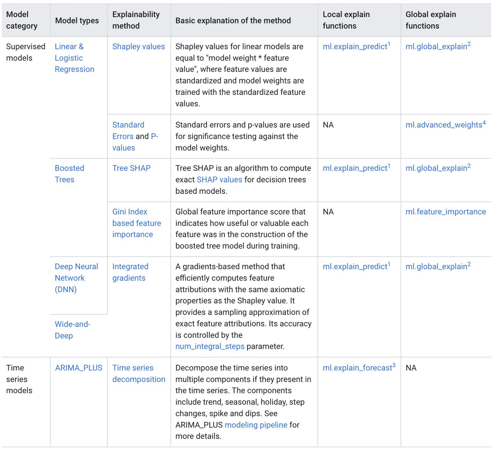
BigQuery Explainable AI applies to a variety of models, including supervised learning models for IID data and time series models. The documentation for BigQuery Explainable AI provides an overview of the different ways of applying explainability per model. Note that each explainability method has its own way of calculation (e.g. Shapley values), which are covered more in-depth in the documentation.
Examples with BigQuery Explainable AI
In this next section, we will show three examples of how to use BigQuery Explainable AI in different ML applications:
Regression models with BigQuery Explainable AI
Let’s use a boosted tree regression model to predict how much a taxi cab driver will receive in tips for a taxi ride, based on features such as number of passengers, payment type, total payment and trip distance. Then let’s use BigQuery Explainable AI to help us understand how the model made the predictions in terms of global explainability (which features were most important?) and local explainability (how did the model arrive at each prediction?).
The taxi trips dataset comes from the BigQuery public datasets and is publicly available in the table: bigquery-public-data.new_york_taxi_trips.tlc_yellow_trips_2018.
First, you can train a boosted tree regression model.
CREATE OR REPLACE MODEL bqml_tutorial.taxi_tip_regression_modelOPTIONS (model_type='boosted_tree_regressor',input_label_cols=['tip_amount'],max_iterations = 50,tree_method = 'HIST',subsample = 0.85,enable_global_explain = TRUE) ASSELECTvendor_id,passenger_count,trip_distance,rate_code,payment_type,total_amount,tip_amountFROM`bigquery-public-data.new_york_taxi_trips.tlc_yellow_trips_2018`WHERE tip_amount >= 0LIMIT 1000000
Now let’s do a prediction using ML.PREDICT, which is the standard way in BigQuery ML to make predictions without explainability.
SELECT *FROMML.PREDICT(MODEL bqml_tutorial.taxi_tip_regression_model,(SELECT"0" AS vendor_id,1 AS passenger_count,CAST(5.85 AS NUMERIC) AS trip_distance,"0" AS rate_code,"0" AS payment_type,CAST(55.56 AS NUMERIC) AS total_amount))

But you might wonder—how did the model generate this prediction of ~11.077?
BigQuery Explainable AI can help us answer this question. Instead of using ML.PREDICT, you use ML.EXPLAIN_PREDICT with an additional optional parameter top_k_features. ML.EXPLAIN_PREDICT extends the capabilities of ML.PREDICT by outputting several additional columns that explain how each feature contributes to the predicted value. In fact, since ML.EXPLAIN_PREDICT includes all the output from ML.PREDICT anyway, you may want to consider using ML.EXPLAIN_PREDICT every time instead.
SELECT *FROMML.EXPLAIN_PREDICT(MODEL bqml_tutorial.taxi_tip_regression_model,(SELECT"0" AS vendor_id,1 AS passenger_count,CAST(5.85 AS NUMERIC) AS trip_distance,"0" AS rate_code,"0" AS payment_type,CAST(55.56 AS NUMERIC) AS total_amount),STRUCT(6 AS top_k_features))
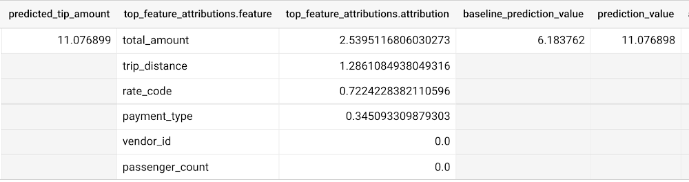
The way to interpret these columns is:
Σfeature_attributions + baseline_prediction_value = prediction_value
Let’s break this down. The prediction_value is ~11.077, which is simply the predicted_tip_amount. The baseline_prediction_value is ~6.184, which is the tip amount for an average instance. top_feature_attributions indicates how much each of the features contributes towards the prediction value. For example, total_amount contributes ~2.540 to the predicted_tip_amount.
ML.EXPLAIN_PREDICT provides local feature explainability for regression models. For global feature importance, see the documentation for ML.GLOBAL_EXPLAIN.
Classification models with BigQuery Explainable AI
Let’s use a logistic regression model to show you an example of BigQuery Explainable AI with classification models. We can use the same public dataset as before: bigquery-public-data.new_york_taxi_trips.tlc_yellow_trips_2018.
Train a logistic regression model to predict the bracket of the percentage of the tip amount out of the taxi bill.
CREATE OR REPLACE MODEL bqml_tutorial.taxi_tip_classification_modelOPTIONS(model_type='logistic_reg',input_label_cols=['tip_bucket'],enable_global_explain=true) ASSELECTvendor_id,passenger_count,trip_distance,rate_code,payment_type,total_amount,CASEWHEN tip_amount > total_amount*0.20 THEN '20% or more'WHEN tip_amount > total_amount*0.15 THEN '15% to 20%'WHEN tip_amount > total_amount*0.10 THEN '10% to 15%'ELSE '10% or less'END AS tip_bucketFROM`bigquery-public-data.new_york_taxi_trips.tlc_yellow_trips_2018`WHERE tip_amount >= 0LIMIT 1000000
Next, you can run ML.EXPLAIN_PREDICT to get both the classification results and the additional information for local feature explainability. For global explainability, you can use ML.GLOBAL_EXPLAIN. Again, since ML.EXPLAIN_PREDICT includes all the output from ML.PREDICT anyway, you may want to consider using ML.EXPLAIN_PREDICT every time instead.
SELECT *FROMML.EXPLAIN_PREDICT(MODEL bqml_tutorial.taxi_tip_classification_model,(SELECT"0" AS vendor_id,1 AS passenger_count,CAST(5.85 AS NUMERIC) AS trip_distance,"0" AS rate_code,"0" AS payment_type,CAST(55.56 AS NUMERIC) AS total_amount),STRUCT(6 AS top_k_features))
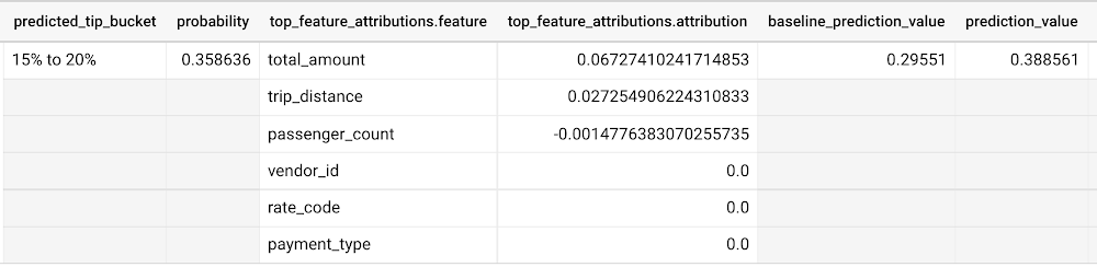
Similar to the regression example earlier, the formula is used to derive the prediction_value:
Σfeature_attributions + baseline_prediction_value = prediction_value
As you can see in the screenshot above, the baseline_prediction_value is ~0.296. total_amount is the most important feature in making this specific prediction, contributing ~0.067 to the prediction_value, though followed by trip_distance. The feature passenger_count contributes negatively to prediction_value by -0.0015. The features vendor_id, rate_code, and payment_type did not seem to contribute much to the prediction_value.
You may wonder why the prediction_value of ~0.389 doesn’t equal the probability value of ~0.359. The reason is that unlike for regression models, for classification models, prediction_value is not a probability score. Instead, prediction_value is the logit value (i.e., log-odds) for the predicted class, which you could separately convert to probabilities by applying the softmax transformation to the logit values. For example, a three-class classification has a log-odds output of [2.446, -2.021, -2.190]. After applying the softmax transformation, the probability of these class predictions is [0.9905, 0.0056, 0.0038].
Time-series forecasting models with BigQuery Explainable AI
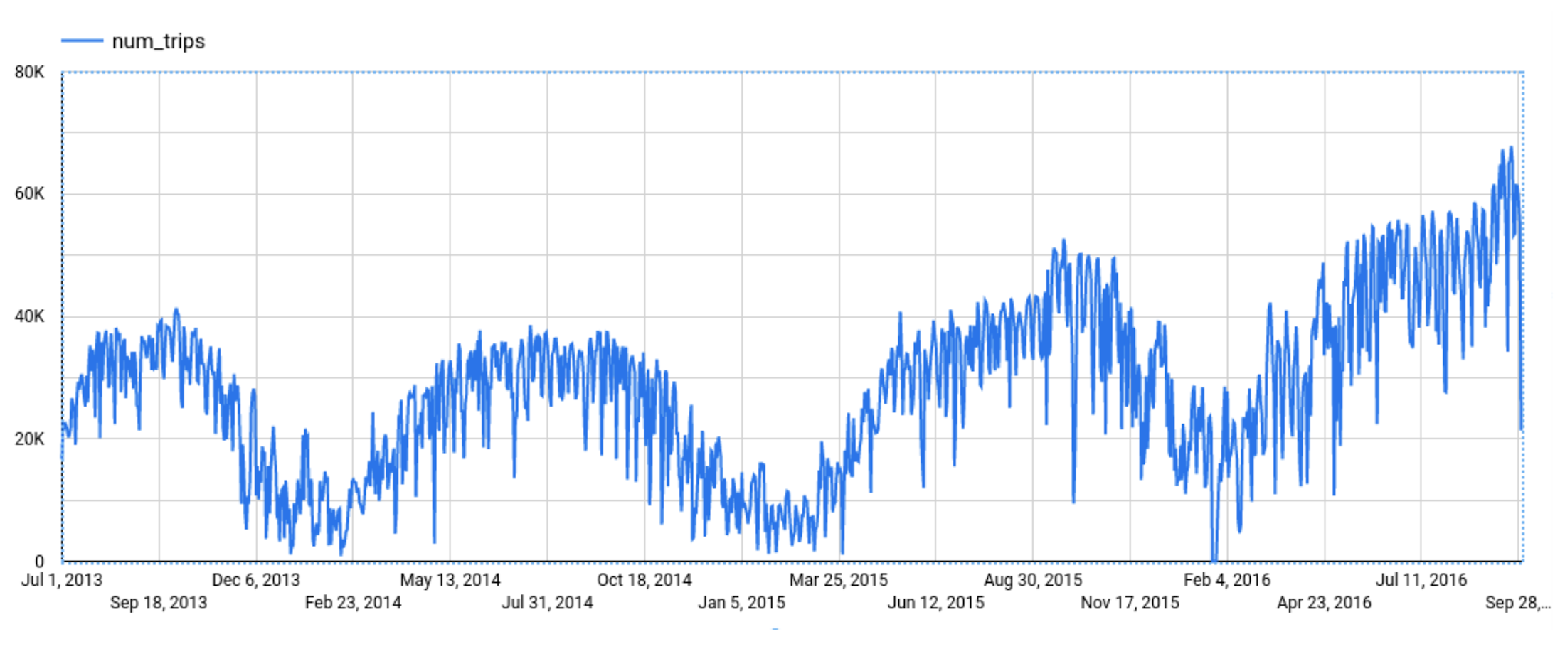
Explainable AI for forecasting provides more interpretability into how the forecasting model came to its predictions. Let’s go through an example of forecasting the number of bike trips in NYC using the new_york.citibike_trips public data in BigQuery.
You can train a time-series model ARIMA_PLUS:
CREATE OR REPLACE MODEL bqml_tutorial.nyc_citibike_arima_modelOPTIONS(model_type = 'ARIMA_PLUS',time_series_timestamp_col = 'date',time_series_data_col = 'num_trips',holiday_region = 'US') ASSELECTEXTRACT(DATE from starttime) AS date,COUNT(*) AS num_tripsFROM`bigquery-public-data.new_york.citibike_trips`GROUP BY dateNext, you can first try forecasting without explainability using ML.FORECAST:SELECT*FROMML.FORECAST(MODEL bqml_tutorial.nyc_citibike_arima_model,STRUCT(365 AS horizon, 0.9 AS confidence_level))
This function outputs the forecasted values and the prediction interval. Plotting it in addition to the input time series gives the following figure.
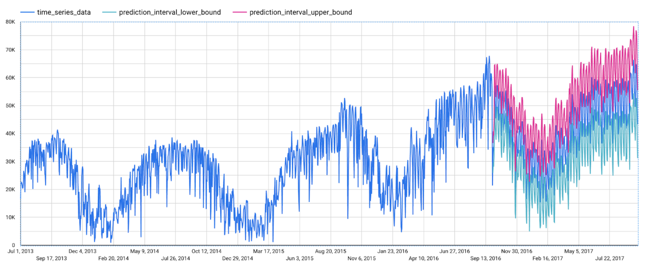
But how does the forecasting model arrive at its predictions? Explainability is especially important if the model ever generates unexpected results.
With ML.EXPLAIN_FORECAST, BigQuery Explainable AI provides extra transparency into the seasonality, trend, holiday effects, level (step) changes, and spikes and dips outlier removal. In fact, since ML.EXPLAIN_FORECAST includes all the output from ML.FORECAST anyway, you may want to consider using ML.EXPLAIN_FORECAST every time instead.
SELECT*FROMML.EXPLAIN_FORECAST(MODEL bqml_tutorial.nyc_citibike_arima_model,STRUCT(365 AS horizon, 0.9 AS confidence_level))
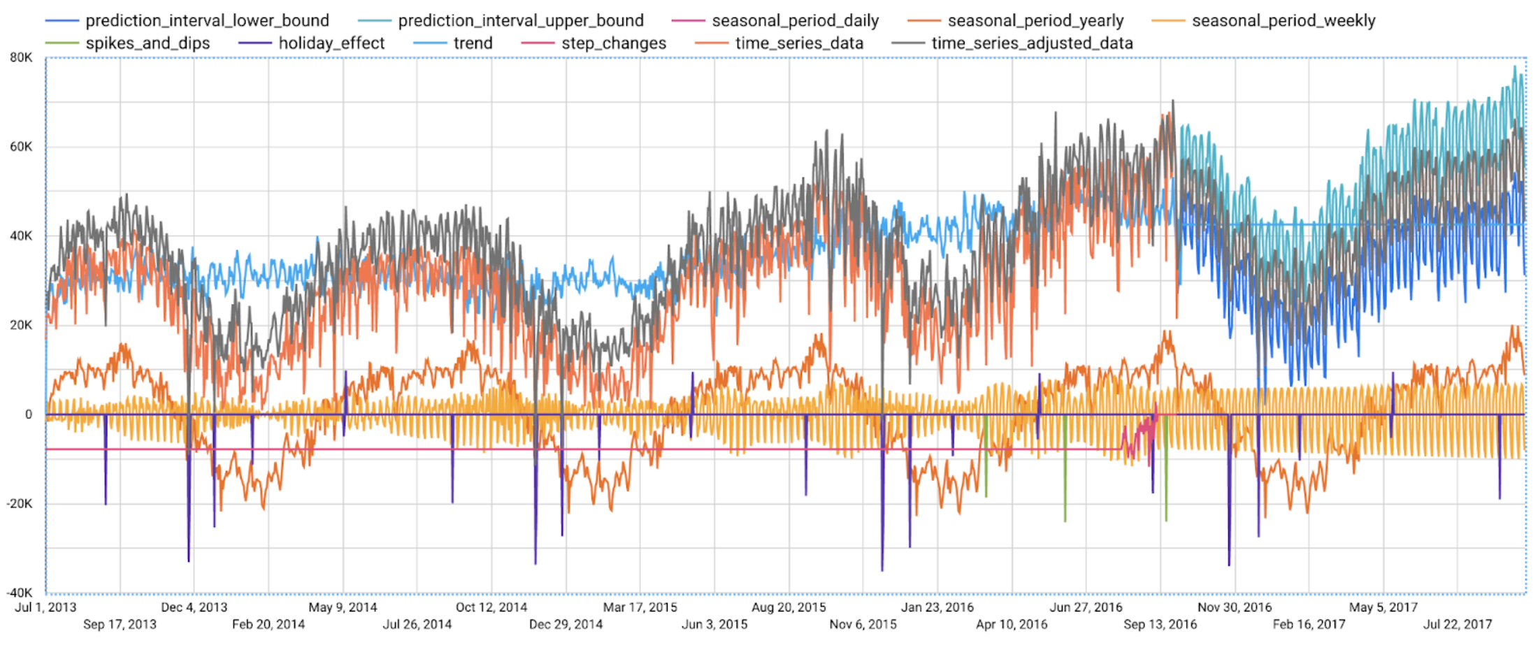
Compared to the previous figure which only shows the forecasting results, this figure shows much richer information to explain how the forecast is made.
First, it shows how the input time series is adjusted by removing the spikes and dips anomalies, and by compensating the level changes. That is:
time_series_adjusted_data = time_series_data - spikes_and_dips - step_changes
Second, it shows how the adjusted input time series is decomposed into different components such as both weekly and yearly seasonal components, holiday effect component and trend component. That is
time_series_adjusted_data = trend + seasonal_period_yearly + seasonal_period_weekly + holiday_effect + residual
Finally, it shows how these components are forecasted separately to compose the final forecasting results. That is:
time_series_data = trend + seasonal_period_yearly + seasonal_period_weekly + holiday_effect
For more information on these time series components, please see the documentation here.
Conclusion
With the GA of BigQuery Explainable AI, we hope you will now be able to interpret your machine learning models with ease.
Thanks to the BigQuery ML team, especially Lisa Yin, Jiashang Liu, Amir Hormati, Mingge Deng, Jerry Ye and Abhinav Khushraj. Also thanks to the Vertex Explainable AI team, especially David Pitman and Besim Avci.
Spot Slow MySQL Queries Fast with Stackdriver Monitoring

4032
Of your peers have already read this article.
4:30 Minutes
The most insightful time you'll spend today!
When you’re serving customers online, speed is essential for a good experience. As the amount of data in a database grows, queries that used to be fast can slow down.
For example, if a query has to scan every row because a table is missing an index, response times that were acceptable with a thousand rows can turn into multiple seconds of waiting once you have a million rows.
If this query is executed every time a user loads your web page, their browsing experience will slow to a crawl, causing user frustration. Slow queries can also impact automated jobs, causing them to time out before completion.
If there are too many of these slow queries executing at once, the database can even run out of connections, causing all new queries, slow or fast, to fail.
The popular open-source databases MySQL and Google Cloud Platform‘s fully managed version, Cloud SQL for MySQL, include a feature to log slow queries, letting you find the cause, then optimize for better performance.
However, developers and database administrators typically only access this slow query log reactively, after users have seen the effects and escalated the performance degradation.
With Stackdriver Logging and Monitoring, you can stay ahead of the curve for database performance with automatic alerts when query latency goes over the threshold, and a monitoring dashboard that lets you quickly pinpoint the specific queries causing the slowdown.
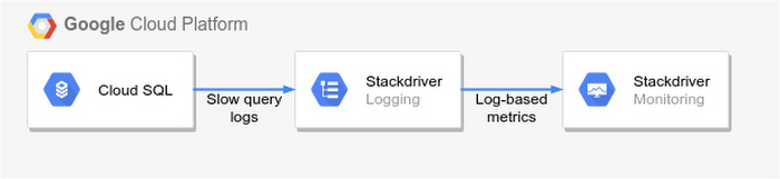
To get started, import MySQL’s slow query log into Stackdriver Logging.
Once the logs are in Stackdriver, it’s straightforward to set up logs-based metrics that can both count the number of slow queries over time, which is useful for setting up appropriate alerts, and also provide breakdowns by slow SQL statement, allowing speedy troubleshooting.
What’s more, this approach works equally well for managed databases in Cloud SQL for MySQL and for self-managed MySQL databases hosted on Compute Engine.
For a step-by-step tutorial to set up slow query monitoring, check out Monitoring slow queries in MySQL with Stackdriver. For more ideas about what else you can accomplish with Stackdriver Logging, check out Design patterns for exporting Stackdriver Logging.
Autoclass: Simplify and Automate Cost Optimization for Cloud Storage

3224
Of your peers have already read this article.
3:00 Minutes
The most insightful time you'll spend today!
There is a data explosion challenge that most IT admins and companies are tackling regularly. The cost-effectiveness, durability and scalability make object storage the first choice for unstructured data. Cloud Storage is an object storage service capable of storing data at exabyte scale and easily managing billions, if not trillions, of objects. However, cost optimization for data stored in object storage is a hard problem.
Choosing the right storage class for your data requires you to know about the access patterns for this data. However, if the access patterns are unknown or unpredictable, it’s often difficult for customers to choose the right storage class for their data. Data placement can have a significant impact on cost as the storage price for the archive class is 6% the storage price for the standard storage class. Having frequently accessed data in colder storage classes can lead to unexpected operations charges. Having data that is never accessed in standard storage can lead to large at-rest storage bills.
As IT administrators and organizations enable different applications and workloads to start leveraging object storage at massive scale, optimizing for cost is only getting exponentially harder to solve. As they migrate workloads to cloud they would like to have predictability and control in their overall storage spend. Wouldn’t it be great if there was a way to automatically place your data in the best storage class?
Introducing Autoclass – a new managed data placement service for Cloud Storage.
Simplifying Lifecycle Management while Reducing TCO
Autoclass is an easy to use bucket-level setting that simplifies and automates lifecycle management of all your Cloud Storage data based on last access time.
This is very useful for workloads with unpredictable and unknown access patterns. It automatically moves data that is not accessed to colder storage classes to reduce at-rest storage cost. When cold data is accessed, it is automatically promoted to Standard storage class to optimize the operations costs for future accesses.
Autoclass automatically delivers cost savings and removes inefficiencies by moving data to the storage class with the most favorable pricing for customer workloads.
It helps organizations achieve price predictability by removing surcharges associated with colder storage classes – there are no early deletion fees, retrieval fees or operations charges for class transitions when Autoclass is enabled on a bucket.
What are customers saying about Autoclass?
“Redivis is a data platform for academic research. We connect data managers with researchers to discover, understand, and analyze Petabytes of data. With Cloud Storage Autoclass, this shifts the paradigm in the research community,” said Ian Matthews, co-founder and CEO of Redivis Inc. “We can now keep more data for longer periods of time while reducing our costs. In fact, I’d estimate 90% of our data will benefit from Autoclass.”
Ian adds “Not only would it cost valuable engineering resources to build cost-optimization ourselves, but it would open us up to potentially costly mistakes in which we incur retrieval charges for prematurely archived data. Autoclass helps us reduce storage costs and achieve price predictability in a simple and automated way.”
Using Autoclass
With this release, Autoclass can be enabled when you create a new Cloud Storage bucket by using CLI, API, or Cloud Console. Once enabled on a bucket, Autoclass will manage the lifecycle of all objects that are uploaded to the bucket until disabled.
If you choose to disable Autoclass, all the objects in the bucket will remain in their current storage class. This disablement doesn’t require any data movement or any changes to storage classes of objects and hence, incurs no charge.
The support for enabling Autoclass on existing Cloud Storage buckets will be available in an upcoming release in 2023.
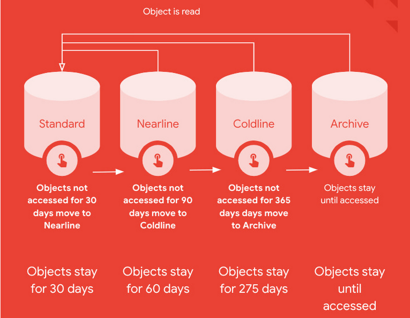
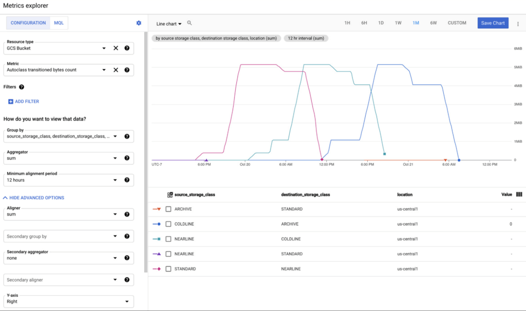
All transitions carried out by Autoclass can be observed using Cloud Monitoring dashboards. This provides easy observability and allows you to validate what Autoclass is doing for your data in an automated way. These dashboards can leverage 2 new Cloud metrics published for Autoclass:
- Number of objects transitioned by Autoclass (autoclass/transition_operation_count)
- Number of bytes transitioned between classes by Autoclass (autoclass/transitioned_bytes_count)
Getting Started
All Cloud Storage customers can enable Autoclass on their new buckets and realize the cost savings for themselves. For more information and detailed instructions on how to enable Autoclass, refer to the documentation here.
Creating and Using Storage Buckets for Your Data Needs

1386
Of your peers have already read this article.
2:30 Minutes
The most insightful time you'll spend today!
So, you want to store objects on the cloud? But you’re really new to Google Cloud or Cloud Storage and would like someone to walk you through the process step by step?
Today is your lucky day!
I will help you understand the big steps involved in setting up and using Cloud Storage. For a walkthrough of all the steps involved that even includes highlighting of things to select so you don’t spend all your time playing “Where’s Waldo” on the page looking for that one button, click try the tutorial!
Creating buckets, storing objects in them, and adjusting permissions may feel challenging at first, but after you’ve walked through these steps, you’ll be able to create and use the Cloud Storage your project needs.
Resource Hierarchy
Projects contain all of the related parts of your application. Inside projects, you may have buckets, the top level containers in Cloud Storage. Files and folders are stored in buckets. You can grant access to a bucket, folder, or file using Identity and Access Management.

You can do all of that in this interactive tutorial. So let’s get started. I suggest you follow along in the tutorial so you can see the specific keys and screens as I describe them.
Creating a project
Everything in your application will be in a project, even if the only service you are using is storage. Projects need to be associated with a billing account, so if you don’t have one, consider signing up for the Free Trial. You’ll start in the Cloud Console.
Creating a bucket
Once you have a project, you can use storage by navigating to the Cloud Storage page by using either the Navigation menu at the top left of the console or by searching for “Cloud Storage” using the search box at the top of the console.
At the Buckets page of Cloud Storage, you’ll be able to create a bucket. The name of your bucket needs to be globally unique; that is no other bucket in Google Cloud Storage can have the same name. This is because if you or your organization allow your bucket to be accessible on the Internet, it will be at the URL https://storage.googleapis.com/<bucket name>. You can also consider implementing a security feature to prevent data exfiltration, organization restriction headers when you’re finished creating your bucket.. Pick a region close to you for your bucket. In some cases it may make sense to use multi-region or dual-region, but the details are more than I want to get into here. Don’t worry; you can find lots more information on them! Additionally, I won’t go into the details about selecting the appropriate storage class based on access frequency and longevity, but more information can be found here as well our recently introduced Autoclass tiering feature..
Since buckets can be accessed from the Internet, you need to be careful to only make the things you want to be public, public. The default value is to keep your data off of the Internet, so when you create the bucket, there’s an option to “Enforce public access prevention on this bucket” that is already selected. Since we’ll be making items in this bucket public later on, clear the option before confirming the bucket information. Don’t worry; you’ll see how to set that option back later.
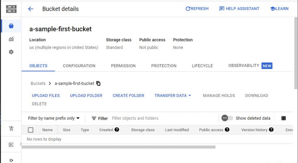
Take a look at the Bucket detail page. There are tabs to see the objects in the bucket, the permissions on the bucket, and much more. There are commands to create folders and to upload files and folders. We’ll do some of this in the next section. You can even find out much more from the Learn option in the upper right.
Adding items to the bucket
Find a file you’d like to upload to this bucket, remembering it will be made public to the Internet later. If you don’t have anything available, there’s a picture of a cat (of course, it’s a cat picture, this is the Internet!) in the interactive tutorial.
Go to the bucket details for your bucket. Using the “Upload files” button, you’ll just upload the file to the bucket by selecting the file from your computer. We won’t get into service classes here, but when you’re ready, there are links in the references.
Of course, if you have a lot of files in a bucket, you probably will want some sort of organization. You can do this by creating folders in your bucket with the “Create Folder” option. Once you’ve done that, you can go to the overflow menu (three vertical dots at the end line with the object information) and select Move. Remember, if you need help finding this, the interactive tutorial will point it out.
Making a bucket public
No surprise, the Bucket details hold lots of information about your bucket. You’ll change the bucket’s permissions in the Permission tab. (I hope that’s not a surprise.) You can then give access to individuals, groups, or all users. For this tutorial, follow the steps to grant access to allUsers. There are a variety of different levels of access you can grant to a user. In this case, just grant the ability to view the object using Storage Object Viewer.
Then go into the Objects tab to find the URL for the object you uploaded. Copy that URL and ensure you can indeed access the object from another tab or incognito window.
Now that you’ve done that, go back to the Permission tab for the bucket and select Prevent Public Access to secure the bucket again.
So, in a nutshell, to make all files in a bucket public, in the Permissions tab:
- Uncheck the option “Remove Public Access Prevention”
- Use Grant Access to give allUsers the Storage Object Viewer role in Cloud Storage.
To make all files in a bucket private, in the Permissions tab select Prevent Public Access.
Cleaning up
There is a charge to keep items in Cloud Storage, so you’ll probably want to delete the object you uploaded by selecting it and pressing Delete. You can delete the bucket in a similar way. The tutorial has details, of course.
While there are lots more details about Cloud Storage, you’ve got the big picture now. Go do something creative and useful with it!
So what now?
If you haven’t walked through the interactive tutorial, give it a try!
Google’s Diversity Annual Report public dataset & BigQuery

3251
Of your peers have already read this article.
3:30 Minutes
The most insightful time you'll spend today!
Since 2014, tech companies have relied on metrics to identify trouble spots, establish baselines, and measure meaningful progress in diversity, including publishing DEI data directly through diversity annual reports. However, as our understanding of DEI has evolved over time each company’s report has diverged, creating a fragmented landscape of industry-wide data. This separation is problematic as no single company’s diversity dataset can solve tech’s DEI challenges. Instead, we need to build industry-wide systemic solutions to create sustainable change, and those start with establishing a common language for DEI data and standardizing and sharing DEI data across tech companies.
The challenge is most companies publish diversity data in a way that makes it difficult to analyze, such as using bar graphs and pie charts. Researchers, as a result, are unable to easily pull the real, detailed data or aggregate and analyze it for their unique needs (e.g. hiring trends for tech vs. nontechnical roles, representation of Asian women in leadership, and more). As we shared in our most recent Diversity Annual Report, external research shows that sustainable change will only come from solutions that encompass the entire tech industry and data transparency is a critical step in this work.
Google’s Diversity Annual Report public dataset & BigQuery
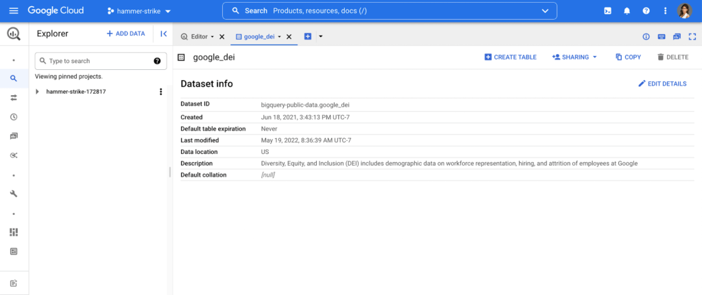
In May, we released our 2022 Diversity Annual Report, which includes demographic data on workforce representation, hiring, and attrition of employees at Google, including leadership. You can see our hiring data by race/ethnicity, gender, and intersectional hiring over time, by region, and more. In an effort to make this data more transparent and accessible for analysis, we have added it as a public dataset in BigQuery, Google Cloud’s powerful data warehousing tool. Our data is now even easier for researchers, community organizations, and industry groups to leverage and compare against external benchmarks to help contextualize our progress.
As one of the first in the industry, we are proud to have published our diversity data on BigQuery for the second year in a row. Our dataset, among others, is public, stored and paid for by Google so those who are interested can use BigQuery’s advanced analytic capabilities through the Google Cloud Public Dataset Program for free*.
Contextualizing diversity data is necessary to make meaningful conclusions
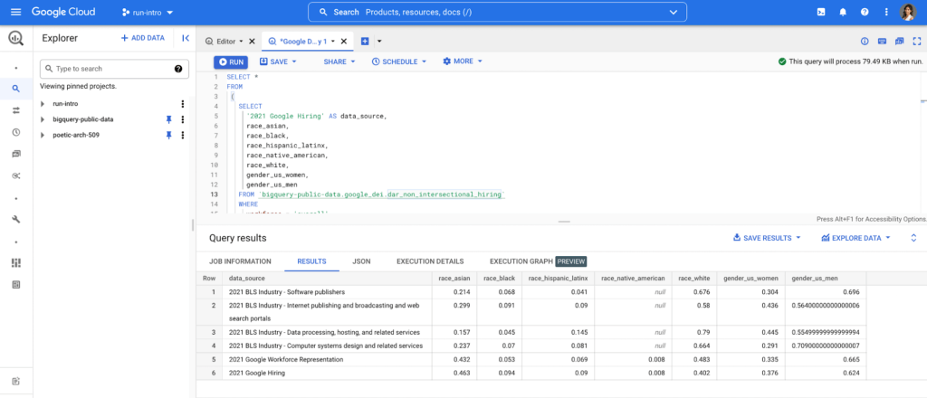
While Google’s diversity dataset can help users compare their own datasets to Google’s current and historical trends, DEI data is only useful when analyzed in the context of other relevant datasets. For example, concluding that Black+ hiring has increased from 8.8% to 9.4% has little meaning unless there is a point of reference, like US general census data, labor force participation rates or graduation rates. It’s why Google also includes other public datasets in BigQuery such as related industry DEI data, talent and graduation pools. By doing so, users can run a sample query that then compares Google’s hiring and representation to related industries (software publishers, data process services, etc.). Users can then better understand and contextualize areas of progress and opportunity, and they can more objectively identify where organizations can take a proactive role in addressing not only DEI in their companies, but also in the communities in which they call home.
Intersectional data and disaggregated baseline metrics
In the workplace, intersectional data is key to understanding the layers of exclusion and inequity that may exist for certain groups. This includes those with social identity overlap, like race, gender, and LGBTQ+, that create multiple levels of inequality or discrimination. It’s critical for DEI data to be disaggregated in a meaningful way to diagnose the true health of a system and to better understand how intersectionality contributes to the greater DEI landscape .
Google’s Diversity Annual Report public dataset includes Google’s intersectional hiring and representation data also broken down by tech, non-tech, and leadership roles. BigQuery’s friendly interface makes it easy to select the relevant parameters and join this data with other public or private datasets to help meaningfully contextualize Google’s data against the broader industry. Anyone from data scientists to DEI stewards can launch public datasets from the Google Cloud Marketplace and start querying them right away. Findings can be visualized through tools like Looker, Data Studio, or Tableau.
This is just the beginning
As DEI work continues to evolve into an industry-wide approach, we must encourage a standard of practice for collecting and reporting data across the board. At scale, data has the power to enable the tech industry to make real improvements collectively, in addition to inside our individual companies. We hope our dataset and sample queries give researchers and individuals a launchpad to become DEI practitioners of the tech industry, and ensure we have the right data to solve the right problems.
Footnote:
*The only time anyone would need to pay is for queries performed on the data after BigQuery’s 1TB/mo of free tier processing. This means that each user receives 1TB of free BigQuery processing every month, which can be used to run queries on this public dataset.
More Relevant Stories for Your Company

Dataplex: Google Cloud’s Intelligent Data Fabric to Manage Data and Analytics at Scale
Enterprises are struggling to make high quality data easily discoverable and accessible for analytics, across multiple silos, to a growing number of people and tools within their organization. They are often forced to make tradeoffs—to move and duplicate data across silos to enable diverse analytics use cases or leave their

Fairygoodboss and Google Cloud Tied to Advancing Diversity and Female Leadership at Workplaces
May is Asian American Pacific Islander Heritage Month — a time for us to come together to celebrate and remember the important people and history of Asian and Pacific Island heritage. This feature highlights founder Georgene Huang and how her startup Fairygodboss uses easy to use Google Cloud tools to

Real-time analytics for on-time delivery: Mercado Libre
Iteration and innovation fuel the data-driven culture at Mercado Libre. In our first post, we presented our continuous intelligence approach, which leverages BigQuery and Looker to create a data ecosystem on which people can build their own models and processes. Using this framework, the Shipping Operations team was able to

Incorporating Custom Holidays into Your Time-Series Models with BigQuery ML
About three years ago, JCB, one of the biggest Japanese payment companies, launched a project to develop new high-value services with agility. We set up a policy of starting small from scratch without using the existing system, which we call the concept of “Dejima”, where we focused on improving various aspects
