After a seamless migration to Google Cloud Platform with CloudCover and Google Cloud Professional Services, Hike has reduced its costs by 20% and processed analytics queries 20 times faster than with its previous cloud provider. The business is also using AI and machine learning to enhance the experience provided by a new sticker-based messaging app, Hike Sticker Chat.

India is a market of opportunity for businesses that provide messaging apps to consumers. With more than 1.3 billion people, the country is the second most populous in the world. However, global messaging app providers face a robust market challenge from Hike, a home-grown internet and technology startup. Launched in 2012, Hike provides innovative products such as Hike Messenger and more recently the AI- and machine-learning-enabled Hike Sticker Chat, a service that enables young people in the country to express themselves through digital stickers.

The business says it understands the people of India and communication like no one else, while its mission is to reduce individuals’ dependency on the keyboard. To do this, Hike is building one of the largest repositories of AI and machine-learning-enabled stickers for Hike Sticker Chat. This messaging platform is, according to Hike, the only product of its type that enables conversations through stickers covering more than 40 languages and local dialects.

Google Cloud Results

• Processes analytics queries 20X faster than previously
• Doubles compute throughput
• Uses Google Cloud Machine Learning Engine managed, distributed capabilities to train complex models on TensorFlow that provide delightful local sticker recommendations through Hike Sticker Chat

Founded by Kavin Bharti Mittal, the Delhi-based venture is backed by SoftBank, Tencent, Tiger Global, Foxconn, and Bharti. To date, Hike has raised $261 million in funding. In August 2016, Hike raised its Series D round of funding, led by Tencent and Foxconn, at a valuation of $1.4 billion. The business is one of the fastest Indian startups to achieve Unicorn status, doing so in less than four years.

Hike started operations on a multinational cloud service. However, as user numbers and usage grew, the business began exploring options to improve performance and stability, reduce costs, and cut administration loads. In particular, Hike wanted to reduce latency between cloud data centers.

Focus on product development

“We aimed to move away from a technology stack with single points of failure to a horizontally scaled, highly reliable, distributed systems and managed services environment that enabled us to focus on product development rather than operations,” says Aditya Gupta, Director, Engineering, Hike.

Hike then began exploring the opportunities presented by Google Cloud Platform. The business held a number of executive-level meetings with Google to understand the capabilities, roadmap, and track record of the cloud service. It then decided to proceed with a proof of concept with Google Cloud Premier Partner CloudCover.

The proof of concept revealed that when Cloud Load Balancing was operating, latency between the Google Cloud data center in Taiwan and Delhi, India, was less than the latency between the incumbent cloud provider’s data center and Delhi. Further, compute throughput was up to two times greater on Compute Engine than on the equivalent service, while Hike could complete more then 1 million connections on Compute Engine – up from 500,000 connections on the incumbent service.

Migrate to GCP

The success of the exercise prompted Hike to migrate its messaging app to Google Cloud Platform. “We chose Google Cloud Platform because of its very broad set of services and features,” explains Gupta. “In addition, Google’s innovation mindset and the richness of the partnership would allow us to be onboarded quickly to machine learning services such as Cloud Machine Learning Engine.”

The business called on Google Cloud Professional Services (Technical Account Management) to help ensure a seamless lift-and-shift migration over two months. Google Cloud Professional Services initially undertook a technical infrastructure kickoff to establish a foundation for architecture requirements such as identity and access management and security.

Google Cloud Professional Services team delivers smooth migration

Google Cloud Professional Services worked closely with Hike to map out and deliver the Google Cloud Platform architecture that would deliver the greatest value to the business. The Professional Services team also worked with Hike to resolve product and support queries quickly; provided project background for product and support teams; and organized project meetings and early adopter program access.

In addition, Professional Services team members worked on site at least once a week, coordinated external support during critical migration periods, and coordinated teams in five countries for a single, 17-hour migration marathon. Over 60 days, the business migrated 7,000 processor cores, running virtual machine instances used for messaging infrastructure and analytics, to Google Cloud Platform.

Throughout the exercise, Google Cloud Professional Services worked with CloudCover to educate the customers’ technology teams to achieve proficiency with Google Cloud Platform. The teams soon built up skills and knowledge of best practices and began applying them to the Google Cloud Platform environment.

The Hike Google Cloud Platform architecture comprises virtual machine instances running in Compute Engine; Cloud Storage for unified object storage; networking; a BigQuery analytics data warehouse; Cloud Dataflow to transform and enrich data; Cloud Load Balancing to distribute workloads to maximize efficiency; and Cloud Dataproc to run Hadoop clusters.

Hike is also stepping up its AI & machine learning capabilities. It uses Google Cloud Machine Learning Engine managed, distributed computing capabilities to train complex models on TensorFlow. This powers key use cases such as delightful local sticker recommendations on Hike Sticker Chat. Hike is also investing heavily on AI and machine learning research.

Hike has achieved a range of benefits from its Google Cloud Platform deployment. As well as reduced latency, improved compute throughput, and increased connection handling, Google Cloud Platform managed services have enabled the business to reduce the time and effort required to administer core infrastructure, with the saved resources allocated to improving its messaging product.

“Managed services are beginning to reduce our operational overheads,” says Gupta. “For example, managed instance groups and Cloud Load Balancing are reducing our instance count and costs, thereby reducing involvement from DevOps and developer teams.”

Google Cloud Platform 20% cheaper

Gupta and his team have calculated that running for three years on Google Cloud Platform will cost, including the cost of migration, 20 percent less than on its previous platform. BigQuery is processing queries 20 times faster than a similar service offered by the previous provider, while storing 125TB of data and streaming 1.5TB of data daily. Furthermore, Hike’s analytics pipeline costs 80 percent less than in its previous environment.

“Google Cloud Platform has played an important role in enabling us to continue to innovate and realize our mission of reducing dependency on the keyboard,” says Gupta.

Editor’s note: We’re inviting partners from across our retail ecosystem to share stories, best practices, and tips and tricks on how they are helping retailers transform during a time that has seen tremendous change. The original version of this blog was published by Trax Retail in October 2021. Please enjoy this updated entry from our partner.

In 2020, we saw a massive leap in online grocery. Within a few weeks, the industry reached numbers that were unexpected for at least four more years. In a snap, what seemed like a relatively insignificant channel became one that grocery retailers simply couldn’t ignore and, what’s more, is likely to remain a norm.

Retailers trying to stay ahead of the curve have already started experimenting with methods like building warehouses and installing robots to fulfill the growing demand, but in-store picking has been and will continue to remain one of the primary methods of fulfilling online orders as it offers several advantages. First, it allows the use of existing infrastructure – large retailers already have geographically well-located outlets in major cities, which enables shorter lead time to delivery. Secondly, it allows retailers to stay flexible and move swiftly between in-store and online order fulfillment. And finally, it fits perfectly with the omnichannel approach to allow customers to shop wherever and however they want – click and collect, curbside pick-up, or inside brick-and-mortar stores.

How improving on-shelf availability helps ecommerce profitability

Despite its many advantages, in-store picking is expensive and affects profitability in an already competitive space since the cost of picking is directly tied with hourly labor fees. Moreover, with labor being a major challenge to obtain and retain, every minute spent picking counts. However, there is an easy way to keep costs down – optimizing the picking process by ensuring product availability and reducing the need for substitution.

An average of 8% of products are not available on-shelf in stores at any given time. As a result, pickers waste much of their time hunting for products that simply aren’t on the shelf or are misplaced, or spend time looking for substitutes, further increasing the time and cost for picking. In fact, grocery pickers often claim that out-of-stock (OOS) occurrences are the main reason that slows down the picking process. Without these factors, pick rates could be two times faster. Since picking accounts for 50% of the fulfillment cost, it has a substantial impact on the order’s bottom line and often makes the difference between a loss-making and a profitable basket.

Maintaining on-shelf availability for the thousands of products in every store has always been a significant problem to solve. The shift to online ordering has made the availability issue even more significant as the shelf is also now the fulfillment center for the majority of online orders. For e-commerce, out of stocks present two major issues for retailers. First, the impact of out-of-stock items is even more noticeable for online shoppers as they do not select their own substitutions. Additionally, out-of-stocks cause inefficiencies in the item fulfillment process, which is already a costly and margin-diluting practice for retailers. The good news is that through a partnership between Trax and Google Cloud, and the power of Google Cloud’s AI/ML capabilities, these challenges are addressed. The granular, real-time data at scale to enable picking efficiency and the data transparency to unlock a better shopping experience are now a reality which benefits both shoppers and store associates.

Trax and Google Cloud technology helps the bottom line

Trax and Google Cloud offer solutions that can help retailers improve on-shelf availability (OSA). Trax Retail Watch powered by Google Cloud uses computer vision (CV) and AI to create a digital version of the physical store in real-time and informs out-of-stocks so that retailers always have full visibility of items that are running low and can replenish them quickly. In turn, pickers are more likely to find everything they need quickly without facing the problem of missing products or having to look for substitutes. Trax Retail Watch also allows store associates to quickly spot any issues arising on shelves without having to physically walk down each aisle. From misplaced products to low stock, having full visibility means that shelf managers make more informed decisions, so that pickers face fewer obstacles, are aware of the true inventory, and significantly improve their pick rates. Faster picking means lower costs and ultimately, higher margins for online grocery orders.

With more e-commerce retailers crowding the online space, competition is tough. Want to know how frustrated e-commerce shoppers are about on-shelf availability? Trax uncovered this problem through an in-depth consumer study. Learn how to address shopper happiness while driving more profitable fulfillment and stay on the leaderboard with this Trax and Google Cloud whitepaper: Winning the online grocery race.

When it comes to anomaly detection, one of the key challenges that many organizations face is that it can be difficult to know how to define what an anomaly is. How do you define and anticipate unusual network intrusions, manufacturing defects, or insurance fraud? If you have labeled data with known anomalies, then you can choose from a variety of supervised machine learning model types that are already supported in BigQuery ML. But what can you do if you don’t know what kind of anomaly to expect, and you don’t have labeled data? Unlike typical predictive techniques that leverage supervised learning, organizations may need to be able to detect anomalies in the absence of labeled data. 

Today we are announcing the public preview of new anomaly detection capabilities in BigQuery ML that leverage unsupervised machine learning to help you detect anomalies without needing labeled data. Depending on whether or not the training data is time series, users can now detect anomalies in training data or on new input data using a new ML.DETECT_ANOMALIES function (documentation), with the following models:

• Autoencoder model, now in Public Preview (documentation)
• K-means model, already GA (documentation)
• ARIMA_PLUS time series model, already GA (documentation)

How does anomaly detection with ML.DETECT_ANOMALIES work?

To detect anomalies in non-time-series data, you can use:

• K-means clustering models: When you use ML.DETECT_ANOMALIES with a k-means model, anomalies are identified based on the value of each input data point’s normalized distance to its nearest cluster. If that distance exceeds a threshold determined by the contamination value provided by the user, the data point is identified as an anomaly. 
• Autoencoder models: When you use ML.DETECT_ANOMALIES with an autoencoder model, anomalies are identified based on the reconstruction error for each data point. If the error exceeds a threshold determined by the contamination value, it is identified as an anomaly. 

To detect anomalies in time-series data, you can use: 

• ARIMA_PLUS time series models: When you use ML.DETECT_ANOMALIES with an ARIMA_PLUS model, anomalies are identified based on the confidence interval for that timestamp. If the probability that the data point at that timestamp occurs outside of the prediction interval exceeds a probability threshold provided by the user, the datapoint is identified as an anomaly.

Below we show code examples of anomaly detection in BigQuery ML for each of the above scenarios.

Anomaly detection with a k-means clustering model

You can now detect anomalies using k-means clustering models, by running ML.DETECT_ANOMALIES to detect anomalies in the training data or in new input data. Begin by creating a k-means clustering model:

Language: SQL

  CREATE MODEL `mydataset.my_kmeans_model`
OPTIONS(
  MODEL_TYPE = 'kmeans',
  NUM_CLUSTERS = 8,
  KMEANS_INIT_METHOD = 'kmeans++'
) AS
SELECT 
  * EXCEPT(Time, Class) 
FROM 
  `bigquery-public-data.ml_datasets.ulb_fraud_detection`;

With the k-means clustering model trained, you can now run ML.DETECT_ANOMALIES to detect anomalies in the training data or in new input data.
To detect anomalies in the training data, use ML.DETECT_ANOMALIES with the same data used during training:

Language: SQL

  SELECT
  *
FROM
  ML.DETECT_ANOMALIES(MODEL `mydataset.my_kmeans_model`,
                      STRUCT(0.02 AS contamination),
                      TABLE `bigquery-public-data.ml_datasets.ulb_fraud_detection`);

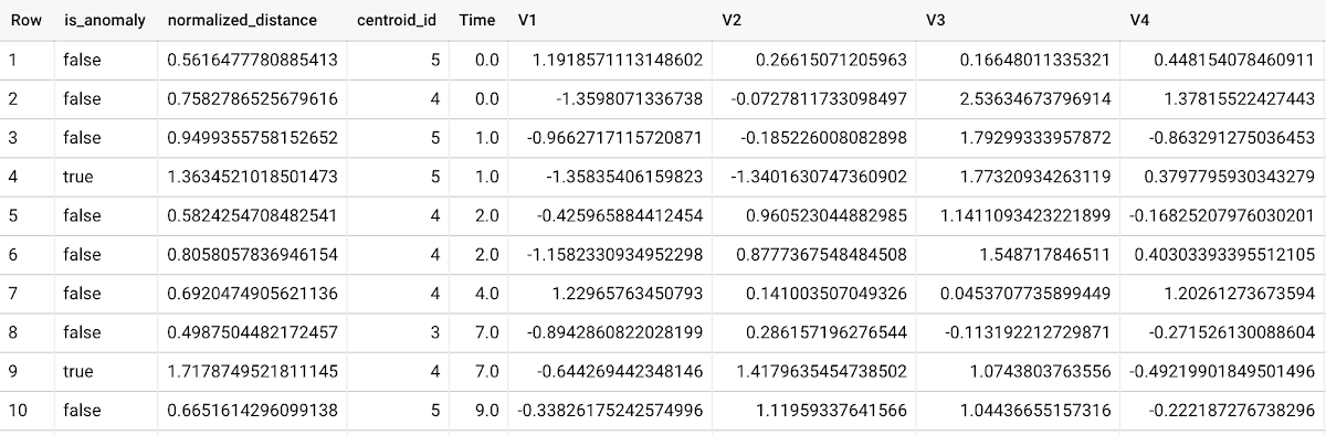
To detect anomalies in new data, use ML.DETECT_ANOMALIES and provide new data as input:

Language: SQL

  SELECT
  *
FROM
  ML.DETECT_ANOMALIES(MODEL `mydataset.my_kmeans_model`,
                      STRUCT(0.02 AS contamination),
                      (SELECT * FROM `mydataset.newdata`));

How does anomaly detection work for k-means clustering models? 

Anomalies are identified based on the value of each input data point’s normalized distance to its nearest cluster, which, if exceeds a threshold determined by the contamination value, is identified as an anomaly. How does this work exactly? With a k-means model and data as inputs, ML.DETECT_ANOMALIES first computes the absolute distance for each input data point to all cluster centroids in the model, then normalizes each distance by the respective cluster radius (which is defined as the standard deviation of the absolute distances of all points in this cluster to the centroid). For each data point, ML.DETECT_ANOMALIES returns the nearest centroid_id based on normalized_distance, as seen in the screenshot above. The contamination value, specified by the user, determines the threshold of whether a data point is considered an anomaly. For example, a contamination value of 0.1 means that the top 10% of descending normalized distance from the training data will be used as the cut-off threshold. If the normalized distance for a datapoint exceeds the threshold, then it is identified as an anomaly. Setting an appropriate contamination will be highly dependent on the requirements of the user or business. 

For more information on anomaly detection with k-means clustering, please see the documentation here.

Anomaly detection with an autoencoder model

You can now detect anomalies using autoencoder models, by running ML.DETECT_ANOMALIES to detect anomalies in the training data or in new input data. 

Begin by creating an autoencoder model:

Language: SQL

  CREATE MODEL `mydataset.my_autoencoder_model`
OPTIONS(
  model_type='autoencoder',
  activation_fn='relu',
  batch_size=8,
  dropout=0.2,  
  hidden_units=[32, 16, 4, 16, 32],
  learn_rate=0.001,
  l1_reg_activation=0.0001,
  max_iterations=10,
  optimizer='adam'
) AS 
SELECT 
  * EXCEPT(Time, Class) 
FROM 
  `bigquery-public-data.ml_datasets.ulb_fraud_detection`;

To detect anomalies in the training data, use ML.DETECT_ANOMALIES with  the same data used during training:

Language: SQL

  SELECT
  *
FROM
  ML.DETECT_ANOMALIES(MODEL `mydataset.my_autoencoder_model`,
                      STRUCT(0.02 AS contamination),
                      TABLE `bigquery-public-data.ml_datasets.ulb_fraud_detection`);

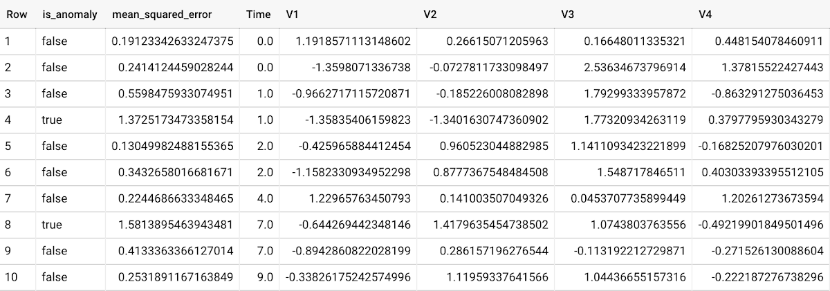
To detect anomalies in new data, use ML.DETECT_ANOMALIES and provide new data as input:

Language: SQL

  SELECT
  *
FROM
  ML.DETECT_ANOMALIES(MODEL `mydataset.my_autoencoder_model`,
                      STRUCT(0.02 AS contamination),
                      (SELECT * FROM `mydataset.newdata`));

How does anomaly detection work for autoencoder models? 

Anomalies are identified based on the value of each input data point’s reconstructed error, which, if exceeds a threshold determined by the contamination value, is identified as an anomaly. How does this work exactly? With an autoencoder model and data as inputs, ML.DETECT_ANOMALIES first computes the mean_squared_error for each data point between its original values and its reconstructed values. The contamination value, specified by the user, determines the threshold of whether a data point is considered an anomaly. For example, a contamination value of 0.1 means that the top 10% of descending error from the training data will be used as the cut-off threshold. Setting an appropriate contamination will be highly dependent on the requirements of the user or business. 

For more information on anomaly detection with autoencoder models, please see the documentation here.

Anomaly detection with an ARIMA_PLUS time-series model

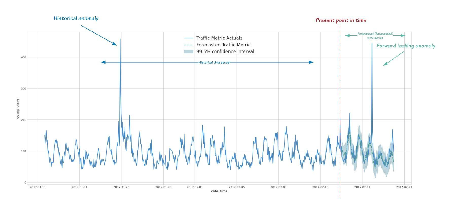
With ML.DETECT_ANOMALIES, you can now detect anomalies using ARIMA_PLUS time series models in the (historical) training data or in new input data. Here are some examples of when might you want to detect anomalies with time-series data:

Detecting anomalies in historical data: 

• Cleaning up data for forecasting and modeling purposes, e.g. preprocessing historical time series before using them to train an ML model.  
• When you have a large number of retail demand time series (thousands of products across hundreds of stores or zip codes), you may want to quickly identify which stores and product categories had anomalous sales patterns, and then perform a deeper analysis of why that was the case.

Forward looking anomaly detection: 

• Detecting consumer behavior and pricing anomalies as early as possible: e.g. if traffic to a specific product page suddenly and unexpectedly spikes, it might be because of an error in the pricing process that leads to an unusually low price. 
• When you have a large number of retail demand time series (thousands of products across hundreds of stores or zip codes), you would like to identify which stores and product categories had anomalous sales patterns based on your forecasts, so you can quickly respond to any unexpected spikes or dips.

How do you detect anomalies using ARIMA_PLUS? Begin by creating an ARIMA_PLUS time series model:

Language: SQL

  CREATE OR REPLACE MODEL mydataset.my_arima_plus_model
OPTIONS(
  MODEL_TYPE='ARIMA_PLUS',
  TIME_SERIES_TIMESTAMP_COL='date',
  TIME_SERIES_DATA_COL='total_amount_sold',
  TIME_SERIES_ID_COL='item_name',
  HOLIDAY_REGION='US' 
) AS
SELECT
  date,
  item_description AS item_name,
  SUM(bottles_sold) AS total_amount_sold
FROM
  `bigquery-public-data.iowa_liquor_sales.sales`
GROUP BY
  date,
  item_name
HAVING
  date BETWEEN DATE('2016-01-04') AND DATE('2017-06-01')
  AND item_name IN ("Black Velvet", "Captain Morgan Spiced Rum",
    "Hawkeye Vodka", "Five O'Clock Vodka", "Fireball Cinnamon Whiskey");

To detect anomalies in the training data, use ML.DETECT_ANOMALIES with the model obtained above:

Language: SQL

  SELECT
  *
FROM
  ML.DETECT_ANOMALIES(MODEL `mydataset.my_arima_plus_model`,
                      STRUCT(0.8 AS anomaly_prob_threshold));

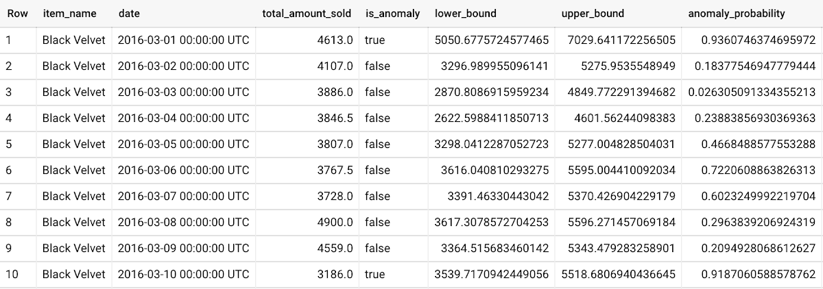
To detect anomalies in new data, use ML.DETECT_ANOMALIES and provide new data as input:

Language: SQL

  WITH
  new_data AS (
  SELECT
    date,
    item_description AS item_name,
    SUM(bottles_sold) AS total_amount_sold
  FROM
    `bigquery-public-data.iowa_liquor_sales.sales`
  GROUP BY
    date,
    item_name
  HAVING
    date BETWEEN DATE('2017-06-02')
    AND DATE('2017-10-01')
    AND item_name IN ('Black Velvet',
      'Captain Morgan Spiced Rum',
      'Hawkeye Vodka',
      "Five O'Clock Vodka",
      'Fireball Cinnamon Whiskey') )
SELECT
  *
FROM
  ML.DETECT_ANOMALIES(MODEL `mydataset.my_arima_plus_model`,
    STRUCT(0.8 AS anomaly_prob_threshold),
    (SELECT
      *
    FROM
      new_data));

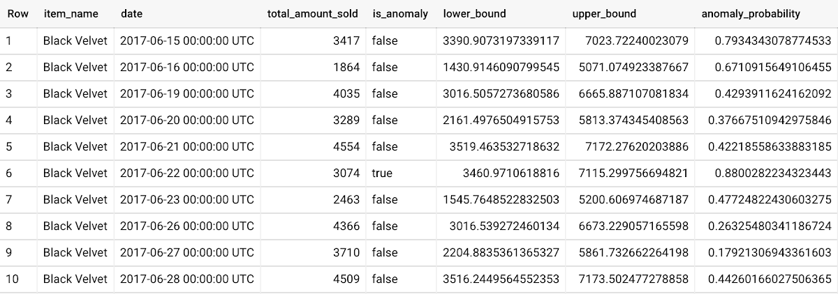
For more information on anomaly detection with ARIMA_PLUS time series models, please see the documentation here.

Thanks to the BigQuery ML team, especially Abhinav Khushraj, Abhishek Kashyap, Amir Hormati, Jerry Ye, Xi Cheng, Skander Hannachi, Steve Walker, and Stephanie Wang.

APIs are the backbone of digital transformation. Via APIs, you can securely share data and functionality with developers both inside and outside of your organizational boundaries, letting you build applications faster, seamlessly connect and interact with partners, and drive new business revenue. 

Because APIs encompass business-critical information, any downtime or performance degradation can lead to significant loss in revenue, customers, and brand value. Therefore, there’s mounting pressure on operations teams to ensure that APIs are always available and performing as expected. If the APIs go down, so too do the services that fuel customer experiences and on which the organization relies for collaboration and business processes.

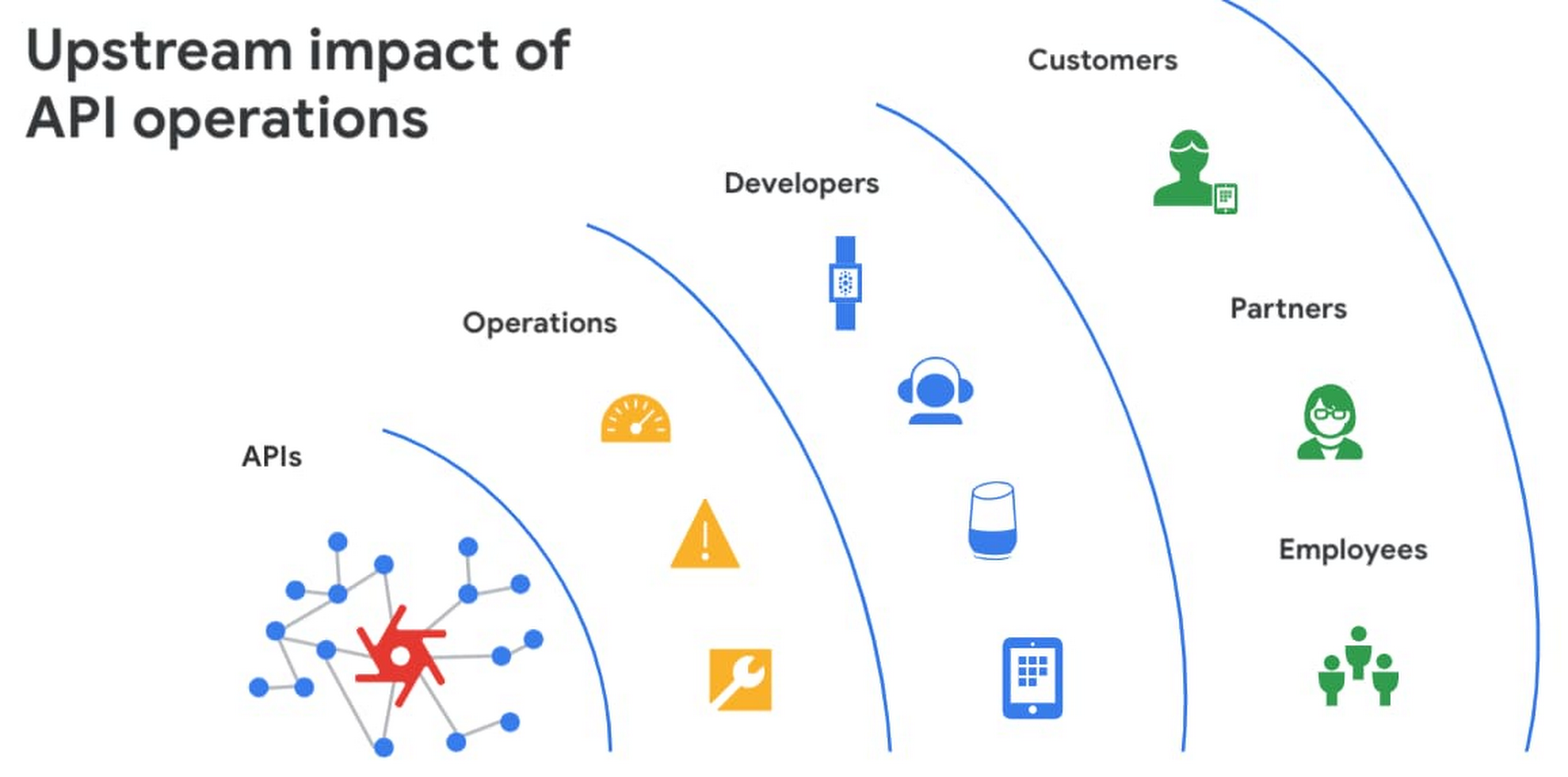
However, as you build and scale your API programs, it becomes practically impossible for API operators to manually monitor and manage all your APIs. To help, we brought the power of industry-leading AI and ML technologies to API operations via Apigee X, a major release of our API management platform. Apigee X seamlessly weaves together Google Cloud’s expertise in AI, security and networking to help you efficiently build and manage APIs at scale. 

Put your API data into action

Apigee applies machine learning to your API metadata and provides you the required tools that simplify various aspects of API operations. A great example of AI for APIs is anomaly detection: 

• AI-powered rules trigger alerts based on a set of predefined conditions that are determined by applying Google’s industry-leading machine learning models to your historical API data.
• Auto-thresholds adjust the monitoring criteria of your APIs and set them to pattern-based values. 
• Reduce overhead results because operators don’t have to manually monitor anomalies or adjust the monitoring thresholds on APIs.

“By applying AI and ML models to our historical API data, these advanced features are able to alert us about scenarios we haven’t thought of. Such automation capabilities significantly reduce our upfront efforts. And from a security perspective, the actionable insights help us ensure that our proxies are exposed only over secure HTTPs ports and adhere to compliance requirements. We’re also able to closely monitor user activity and quickly pull out reports during audits.” – Adam Brancato, Sr. Manager, Global Technology and Security at Citrix

As our customers scale their API programs, they find it extremely useful to harness AI-powered capabilities.  In our recent State of the API Economy 2021 report, we found a 230% increase in enterprises’ use of anomaly detection, bot protection, and security analytics features.

To learn more about Apigee X, and see AI and machine learning in action, check out this video, and to try Apigee X for free, click here.

As Googlers transitioned to working from home during the pandemic, more and more turned to chat-based support to help them fix technical problems. Google’s IT support team looked at many options to help us meet the increased demand for tech support quickly and efficiently. 

More staff? Not easy during a pandemic. 

Let service levels drop? Definitely not. 

Outsource? Not possible with our IT requirements. 

Automation? Maybe, just maybe…

How could we use AI to scale up our support operations, making our team more efficient?

The answer: Smart Reply, a technology developed by a Google Research team with expertise in machine learning, natural language understanding, and conversation modeling. This product provided us with an opportunity to improve our agents’ ability to respond to queries from Googlers by using our corpus of chat data.  Smart Reply trains a model that provides suggestions to techs in real time. This reduces the cognitive load when multi-chatting and helps a tech drive sessions towards resolution.

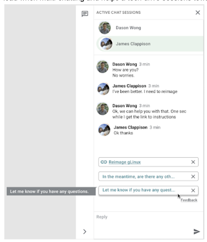
In the solution detailed below, our hope is that IT teams in a similar situation can find best practices and a few shortcuts to implementing the same kind of time saving solutions. Let’s get into it!

Challenges in preparing our data

Our tech support service for Google employees—Techstop—provides a complex service, offering support for a range of products and technology stacks through chat, email, and other channels. 

Techstop has a lot of data. We receive hundreds of thousands of requests for help per year. As Google has evolved we’ve used a single database for all internal support data, storing it as text, rather than as protocol buffers. Not so good for model training. To protect user privacy, we want to ensure no PII (personal identifiable information – e.g. usernames, real names, addresses, or phone numbers) makes it into the model.

To address these challenges we built a FlumeJava pipeline that takes our text and splits each message sent by agent and requester into individual lines, stored as repeated fields in a protocol buffer. As our pipe is executing this task, it also sends text to the Google Cloud DLP API, removing personal information from the session text, replacing it with a redaction that we can later use on our frontend. 

With the data prepared in the correct format, we are able to begin our model training. The model provides next message suggestions for techs based on the overall context of the conversation. To train the model we implemented tokenization, encoding, and dialogue attributes.

Splitting it up

The messages between the agent and customer are tokenized: broken up into discrete chunks for easier use. This splitting of text into tokens must be carefully considered for several reasons:

• Tokenization determines the size of the vocabulary needed to cover the text.
• Tokens should attempt to split along logical boundaries, aiming to extract the meaning of the text.
• Tradeoffs can be made between the size of each token, with smaller tokens increasing processing requirements but enabling easier correlation between different spans of text.

There are many ways to tokenize text (SAFT, splitting on white spaces, etc.), here we chose sentence piece tokenization, with each token referring to a word segment. 

Prediction with encoders

Training the neural network with tokenized values has gone through several iterations. The team used an Encoder-Decoder architecture that took a given vector along with a token and used a softmax function to predict the probability that the token was likely to be the next token in the sentence/conversation. Below, a diagram represents this method using LSTM-based recurrent networks. The power of this type of encoding comes from the ability of the encoder to effectively predict not just the next token, but the next series of tokens.

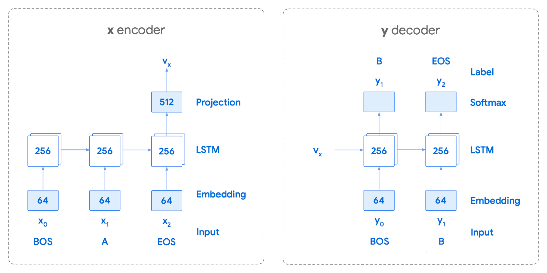
This has proven very useful for Smart Reply. In order to find the optimal sequence, an exponential search over each tree of possible future tokens is required. For this we opted to use beam search over a fixed-size list of best candidates, aiming to avoid increasing the overall memory use and run time for returning a list of suggestions. To do this we arranged tokens in a trie, and used a number of post processing techniques, as well as calculating a heuristic max score for a given candidate, to reduce the time it takes to iterate through the entire token list. While this improves the run time, the model tends to prefer shorter sequences. 

In order to help reduce latency and improve control we decided to move to an Encoder-Encoder architecture. Instead of predicting a single next token and decoding a sequence of following predictions with multiple calls to the model, it instead encodes a candidate sequence with the neural network.

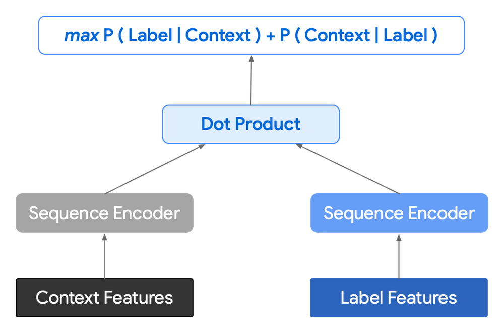
In practice, the two vectors – the context encoding and the encoding of a single candidate output – are combined with dot product to arrive at a score for the given candidate. The goal of this network is to maximize the score for true candidates – e.g. candidates that did appear in the training set – and minimize false candidates.

Choosing how to sample negatives affects the model training greatly. Below are some strategies that can be employed:

• Using positive labels from other training examples in the batch.
• Drawing randomly from a set of common messages. This assumes that the empirical probability of each message is sampled correctly. 
• Using messages from context.
• Generating negatives from another model.

As this encoding generates a fixed list of candidates that can be precomputed and stored, each time a prediction is needed, only the context encoding needs to be computed, then multiplied by the matrix of candidate embeddings. This reduces both the time from the beam search method and the inherent bias towards shorter responses.

Dialogue Attributes

Conversations are more than simple text modeling. The overall flow of the conversation between participants provides important information, changing the attributes of each message. The context, such as who said what to whom and when, offers useful bits of input for the model when making a prediction. To that end the model uses the following attributes during its prediction:

• Local User ID’s – we set a finite number of participants for a given conversation to represent the turn taking between messages, assigning values to those participants. In most cases for support sessions there are 2 participants, requiring ID 0, and 1.
• Replies vs continuations – initially modeling focused only on replies. However, in practice conversations also include instances where participants are following up on the previously sent message. Given this, the model is trained for both same-user suggestions and “other” user suggestions.
• Timestamps  – gaps in conversation can indicate a number of different things. From a support perspective, gaps may indicate that the user has disconnected. The model takes this information and focuses on the time elapsed between messages, providing different predictions based on the values. 

Post processing

Suggestions can then be manipulated to get a more desirable final ranking. Such post-processing includes:

1. Preferring longer suggestions by adding a token factor, generated by multiplying the number of tokens in the current candidate.
2. Demoting suggestions with a high level of overlap with previously sent messages.
3. Promoting more diverse suggestions based on embedding distance similarities.

To help us tune and focus on the best responses the team created a priority list. This gives us the opportunity to influence the model’s output, ensuring that responses that are incorrect can be de-prioritized. Abstractly it can be thought of as a filter that can be calibrated to best suit the client’s needs. 

Getting suggestions to agents

With our model ready we now needed to get it in the hands of our techs. We wanted our solution to be as agnostic to our chat platform as possible, allowing us to be agile when facing tooling changes and speeding up our ability to deploy other efficiency features. To this end we wanted an API that we could query either via gRPC or via HTTPs. We designed a Google Cloud API, responsible for logging usage as well as acting as a bridge between our model and a Chrome Extension we would be using as a frontend.

The hidden step, measurement

Once we had our model, infrastructure, and extension in place we were left with the big question for any IT project. What was our impact? One of the great things about working in IT at Google is that it’s never dull. We have constant changes, be it planned or unplanned. However, this does complicate measuring the success of a deployment like this. Did we improve our service or was it just a quiet month?

In order to be satisfied with our results we conducted an A/B experiment, with some of our techs using our extension, and the others not. The groups were chosen at random with a distribution of techs across our global team, including a mix of techs with varying levels of experience ranging from 3 to 26 months. 

Our primary goal was to measure tech support efficiency when using the tool. We looked at two key metrics as proxies for tech efficiency: 

1. The overall length of the chat. 
2. The number of messages sent by the tech.

Evaluating our experiment

To evaluate our data we used a two-sample permutation test. We had a null hypothesis that techs using the extension would not have a lower time-to-resolution, or be able to send more messages, than those without the extension. The alternative hypothesis was that techs using the extension would be able to resolve sessions quicker or send more messages in approximately the same time.

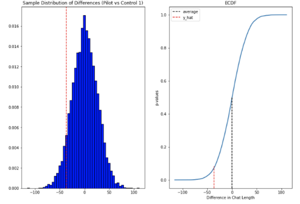
We took the mid mean of our data, using pandas to trim outliers greater than 3 standard deviations away. As the distribution of our chat lengths is not normal, with significant right skew caused by a long tail of longer issues, we opted to measure the difference in means, relying on central limit theorem (CLT) to provide us with our significance values. Any result with a p-value between 1.0 and 9.0 would be rejected. 

Across the entire pool we saw a decrease in chat lengths of 36 seconds.

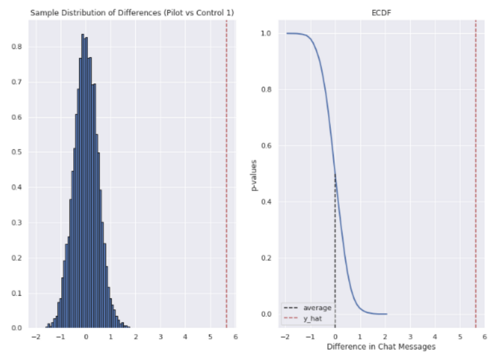
In reference to the number of chat messages we saw techs on average being able to send 5-6 messages more in less time. 

In short, we saw techs were able to send more messages in a shorter period of time. Our results also showed that these improvements increased with support agent tenure, and our more senior techs were able to save an average of ~4 minutes per support interaction.

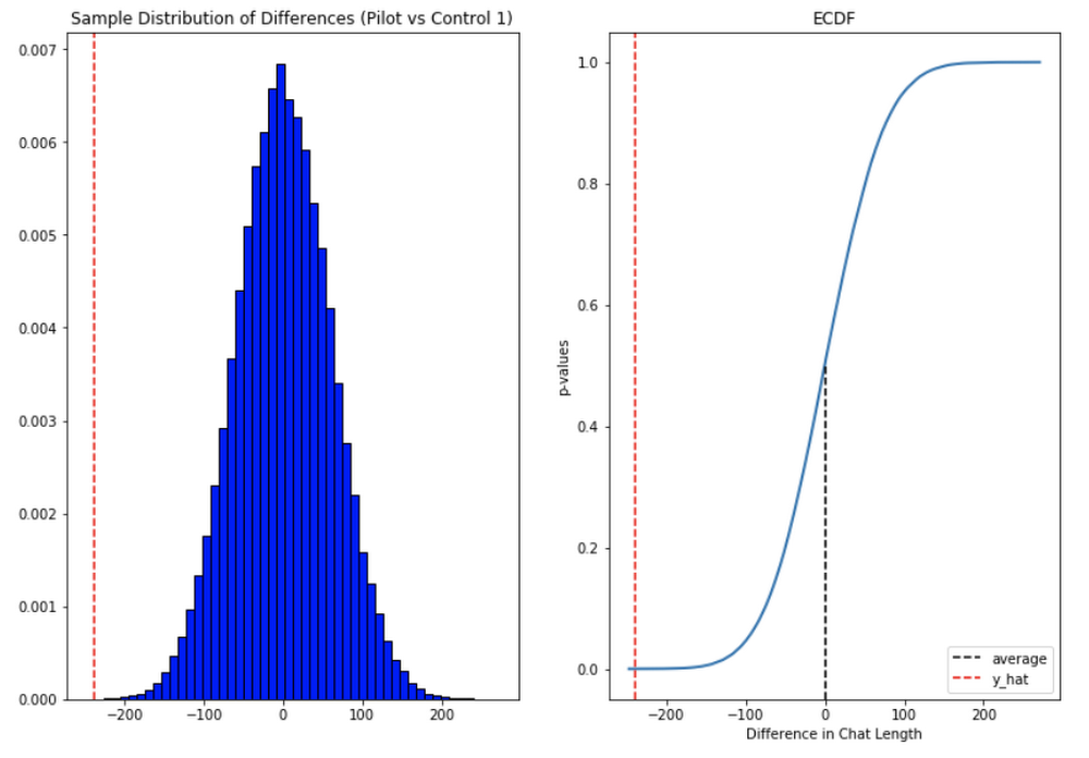
Overall we were pleased with the results. While things weren’t perfect, it looked like we were onto a good thing.

So what’s next for us?

Like any ML project, the better the data the better the result. We’ll be spending time looking into how to provide canonical suggestions to our support agents by clustering results coming from our allow list. We also want to investigate ways of making improvements to the support articles provided by the model, as anything that helps our techs, particularly the junior ones, with discoverability will be a huge win for us.

How can you do this?

A successful applied AI project always starts with data. Begin by gathering the information you have, segmenting it up, and then starting to process it. The interaction data you feed in will determine the quality of the suggestions you get, so make sure you select for the patterns you want to reinforce.

Our Contact Center AI allows tokenization, encoding and reporting, without you needing to design or train your own model, or create your own measurements. It handles all the training for you, once your data is formatted properly. 

You’ll still need to determine how best to integrate its suggestions to your support system’s front-end. We also recommend doing statistical modeling to find out if the suggestions are making your support experience better. 

As we gave our technicians ready-made replies to chat interactions, we saved time for our support team. We hope you’ll try using these methods to help your support team scale.