





Why and How to Migrate to Google BigQuery

5373
Of your peers have already read this article.
6:30 Minutes
The most insightful time you'll spend today!
Over the past few decades, organizations have mastered the science of data warehousing. They have increasingly applied descriptive analytics to large quantities of stored data, gaining insight into their core business operations. Conventional Business Intelligence (BI), which focuses on querying, reporting, and Online Analytical Processing, might have been a differentiating factor in the past, either making or breaking a company, but it’s no longer sufficient.
Today, not only do organizations need to understand past events using descriptive analytics, they need predictive analytics, which often uses machine learning (ML) to extract data patterns and make probabilistic claims about the future. The ultimate goal is to develop prescriptive analytics that combine lessons from the past with predictions about the future to automatically guide real-time actions.
Traditional data warehouse practices capture raw data from various sources, which are often Online Transactional Processing (OLTP) systems. Then, a subset of data is extracted in batches, transformed based on a defined schema, and loaded into the data warehouse. Because traditional data warehouses capture a subset of data in batches and store data based on rigid schemas, they are unsuitable for handling real-time analysis or responding to spontaneous queries. Google designed BigQuery in part in response to these inherent limitations.
Innovative ideas are often slowed by the size and complexity of the IT organization that implements and maintains these traditional data warehouses. It can take years and substantial investment to build a scalable, highly available, and secure data warehouse architecture. BigQuery offers sophisticated software as a service (SaaS) technology that can be used for serverless data warehouse operations. This lets you focus on advancing your core business while delegating infrastructure maintenance and platform development to Google Cloud.
BigQuery offers access to structured data storage, processing, and analytics that’s scalable, flexible, and cost effective. These characteristics are essential when your data volumes are growing exponentially—to make storage and processing resources available as needed, as well as to get value from that data. Furthermore, for organizations that are just starting with big data analytics and machine learning, and that want to avoid the potential complexities of on-premises big data systems, BigQuery offers a pay-as-you-go way to experiment with managed services.
With BigQuery, you can find answers to previously intractable problems, apply machine learning to discover emerging data patterns, and test new hypotheses. As a result, you have timely insight into how your business is performing, which enables you to modify processes for better results. In addition, the end user’s experience is often enriched with relevant insights gleaned from big data analysis, as we explain later in this series.
The migration framework
Undertaking a migration can be a complex and lengthy endeavor. Therefore, we recommend adhering to a framework to organize and structure the migration work in phases:
- Prepare and discover: Prepare for your migration with workload and use case discovery.
- Assess and plan: Assess and prioritize use cases, define measures of success, and plan your migration.
- Execute: Iterate the following steps for each use case:
- Migrate (offload): Migrate only your data, schema, and downstream business applications.
- Migrate (full): Alternatively, migrate the use case fully end-to-end. The same as Migrate (offload), with the addition of the upstream data pipelines.
- Verify and validate: Test and validate the migration to assess return on investment.
The following diagram illustrates the recommended framework and shows how the different phases are connected:

For a deeper understanding, read Migrating data warehouses to BigQuery: Introduction and overview
6183
Of your peers have already watched this video.
18:00 Minutes
The most insightful time you'll spend today!
An Overview of Google’s Data Cloud
Data access, management and privacy has been at the center of priorities for enterprises that are aiming to be more agile, reliable and data-driven. Google Cloud’s technology innovations spanning products like BigQuery, Spanner, Looker and VertexAI help organizations navigate the complexities related to siloed data in large volumes sprawled across databases, data lakes, data warehouses, and data marts in multiple clouds and on-premises. Watch the video to learn how companies are building data on Google Cloud for better analysis, security and management to achieve bottomline!
7476
Of your peers have already watched this video.
1:15 Minutes
The most insightful time you'll spend today!
An Indian Example of How to Really Up Your Customer Experience Game and Increase Conversion Rates With AI
How about selfie analysis of users to recommend them the right lipstick color?
That’s just one of the many ideas folks at Purplle.com came up with to improve the buying experience of Indian consumers.
And without the power of Google Cloud, it would probably have remained just that…an idea.
But today, thanks to Google Cloud, “Nothing seems impossible,” says Suyash Katyayani, CTO, Purplle.
Purplle.com is an online e-commerce company in India and one of the pioneers in creating a digitally-native beauty brands in India.
“The beauty industry is so data intensive that we needed to have a strong data strategy and we were looking out for solutions which would enable us to have a strong data pipeline and a strong data warehousing solution,” says Katyayani.
That’s when it turned to Google Cloud.
Additionally, Purplle.com, says Katyayani, does not have to worry about at what scale the company operates at because they have access to state-of-the-art infrastructure from Google Cloud available to them so that their developers can run experiments.
“The biggest plus point for us has been the agility that Google Cloud has added,” says Katyayani.
New Capabilities in BigQuery to Ease Anomalies Detection in the Absence of Labeled Data

6336
Of your peers have already read this article.
4:00 Minutes
The most insightful time you'll spend today!
When it comes to anomaly detection, one of the key challenges that many organizations face is that it can be difficult to know how to define what an anomaly is. How do you define and anticipate unusual network intrusions, manufacturing defects, or insurance fraud? If you have labeled data with known anomalies, then you can choose from a variety of supervised machine learning model types that are already supported in BigQuery ML. But what can you do if you don’t know what kind of anomaly to expect, and you don’t have labeled data? Unlike typical predictive techniques that leverage supervised learning, organizations may need to be able to detect anomalies in the absence of labeled data.
Today we are announcing the public preview of new anomaly detection capabilities in BigQuery ML that leverage unsupervised machine learning to help you detect anomalies without needing labeled data. Depending on whether or not the training data is time series, users can now detect anomalies in training data or on new input data using a new ML.DETECT_ANOMALIES function (documentation), with the following models:
- Autoencoder model, now in Public Preview (documentation)
- K-means model, already GA (documentation)
- ARIMA_PLUS time series model, already GA (documentation)
How does anomaly detection with ML.DETECT_ANOMALIES work?
To detect anomalies in non-time-series data, you can use:
- K-means clustering models: When you use
ML.DETECT_ANOMALIESwith a k-means model, anomalies are identified based on the value of each input data point’s normalized distance to its nearest cluster. If that distance exceeds a threshold determined by the contamination value provided by the user, the data point is identified as an anomaly. - Autoencoder models: When you use
ML.DETECT_ANOMALIESwith an autoencoder model, anomalies are identified based on the reconstruction error for each data point. If the error exceeds a threshold determined by the contamination value, it is identified as an anomaly.
To detect anomalies in time-series data, you can use:
- ARIMA_PLUS time series models: When you use
ML.DETECT_ANOMALIESwith an ARIMA_PLUS model, anomalies are identified based on the confidence interval for that timestamp. If the probability that the data point at that timestamp occurs outside of the prediction interval exceeds a probability threshold provided by the user, the datapoint is identified as an anomaly.
Below we show code examples of anomaly detection in BigQuery ML for each of the above scenarios.
Anomaly detection with a k-means clustering model
You can now detect anomalies using k-means clustering models, by running ML.DETECT_ANOMALIES to detect anomalies in the training data or in new input data. Begin by creating a k-means clustering model:
Language: SQL
CREATE MODEL `mydataset.my_kmeans_model`OPTIONS(MODEL_TYPE = 'kmeans',NUM_CLUSTERS = 8,KMEANS_INIT_METHOD = 'kmeans++') ASSELECT* EXCEPT(Time, Class)FROM`bigquery-public-data.ml_datasets.ulb_fraud_detection`;
With the k-means clustering model trained, you can now run ML.DETECT_ANOMALIES to detect anomalies in the training data or in new input data.
To detect anomalies in the training data, use ML.DETECT_ANOMALIES with the same data used during training:
Language: SQL
SELECT*FROMML.DETECT_ANOMALIES(MODEL `mydataset.my_kmeans_model`,STRUCT(0.02 AS contamination),TABLE `bigquery-public-data.ml_datasets.ulb_fraud_detection`);
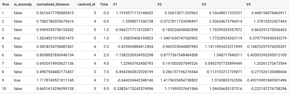
To detect anomalies in new data, use ML.DETECT_ANOMALIES and provide new data as input:
Language: SQL
SELECT*FROMML.DETECT_ANOMALIES(MODEL `mydataset.my_kmeans_model`,STRUCT(0.02 AS contamination),(SELECT * FROM `mydataset.newdata`));

How does anomaly detection work for k-means clustering models?
Anomalies are identified based on the value of each input data point’s normalized distance to its nearest cluster, which, if exceeds a threshold determined by the contamination value, is identified as an anomaly. How does this work exactly? With a k-means model and data as inputs, ML.DETECT_ANOMALIES first computes the absolute distance for each input data point to all cluster centroids in the model, then normalizes each distance by the respective cluster radius (which is defined as the standard deviation of the absolute distances of all points in this cluster to the centroid). For each data point, ML.DETECT_ANOMALIES returns the nearest centroid_id based on normalized_distance, as seen in the screenshot above. The contamination value, specified by the user, determines the threshold of whether a data point is considered an anomaly. For example, a contamination value of 0.1 means that the top 10% of descending normalized distance from the training data will be used as the cut-off threshold. If the normalized distance for a datapoint exceeds the threshold, then it is identified as an anomaly. Setting an appropriate contamination will be highly dependent on the requirements of the user or business.
For more information on anomaly detection with k-means clustering, please see the documentation here.
Anomaly detection with an autoencoder model
You can now detect anomalies using autoencoder models, by running ML.DETECT_ANOMALIES to detect anomalies in the training data or in new input data.
Begin by creating an autoencoder model:
Language: SQL
CREATE MODEL `mydataset.my_autoencoder_model`OPTIONS(model_type='autoencoder',activation_fn='relu',batch_size=8,dropout=0.2,hidden_units=[32, 16, 4, 16, 32],learn_rate=0.001,l1_reg_activation=0.0001,max_iterations=10,optimizer='adam') ASSELECT* EXCEPT(Time, Class)FROM`bigquery-public-data.ml_datasets.ulb_fraud_detection`;
To detect anomalies in the training data, use ML.DETECT_ANOMALIES with the same data used during training:
Language: SQL
SELECT*FROMML.DETECT_ANOMALIES(MODEL `mydataset.my_autoencoder_model`,STRUCT(0.02 AS contamination),TABLE `bigquery-public-data.ml_datasets.ulb_fraud_detection`);
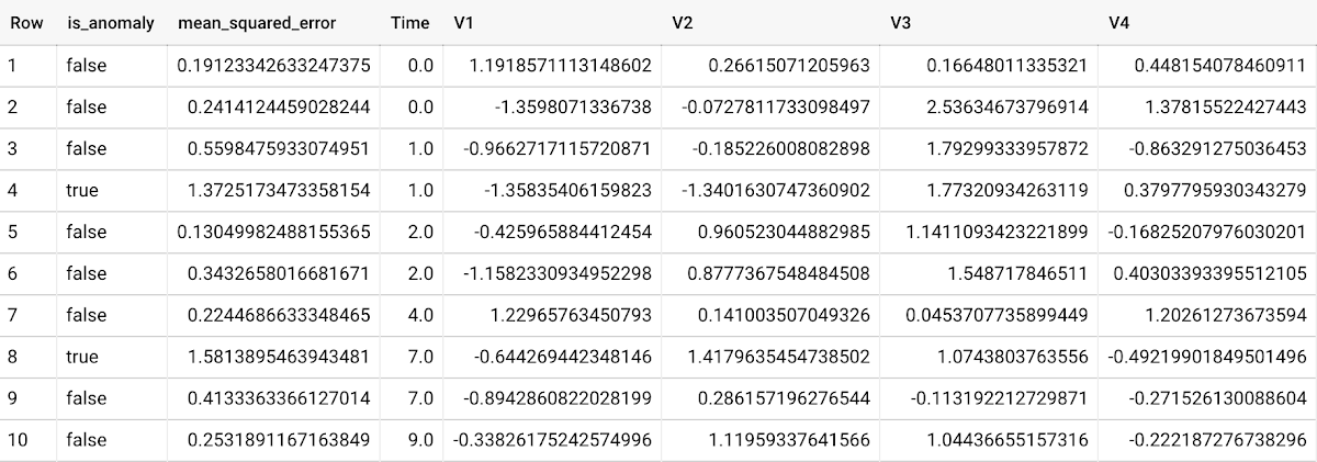
To detect anomalies in new data, use ML.DETECT_ANOMALIES and provide new data as input:
Language: SQL
SELECT*FROMML.DETECT_ANOMALIES(MODEL `mydataset.my_autoencoder_model`,STRUCT(0.02 AS contamination),(SELECT * FROM `mydataset.newdata`));

How does anomaly detection work for autoencoder models?
Anomalies are identified based on the value of each input data point’s reconstructed error, which, if exceeds a threshold determined by the contamination value, is identified as an anomaly. How does this work exactly? With an autoencoder model and data as inputs, ML.DETECT_ANOMALIES first computes the mean_squared_error for each data point between its original values and its reconstructed values. The contamination value, specified by the user, determines the threshold of whether a data point is considered an anomaly. For example, a contamination value of 0.1 means that the top 10% of descending error from the training data will be used as the cut-off threshold. Setting an appropriate contamination will be highly dependent on the requirements of the user or business.
For more information on anomaly detection with autoencoder models, please see the documentation here.
Anomaly detection with an ARIMA_PLUS time-series model
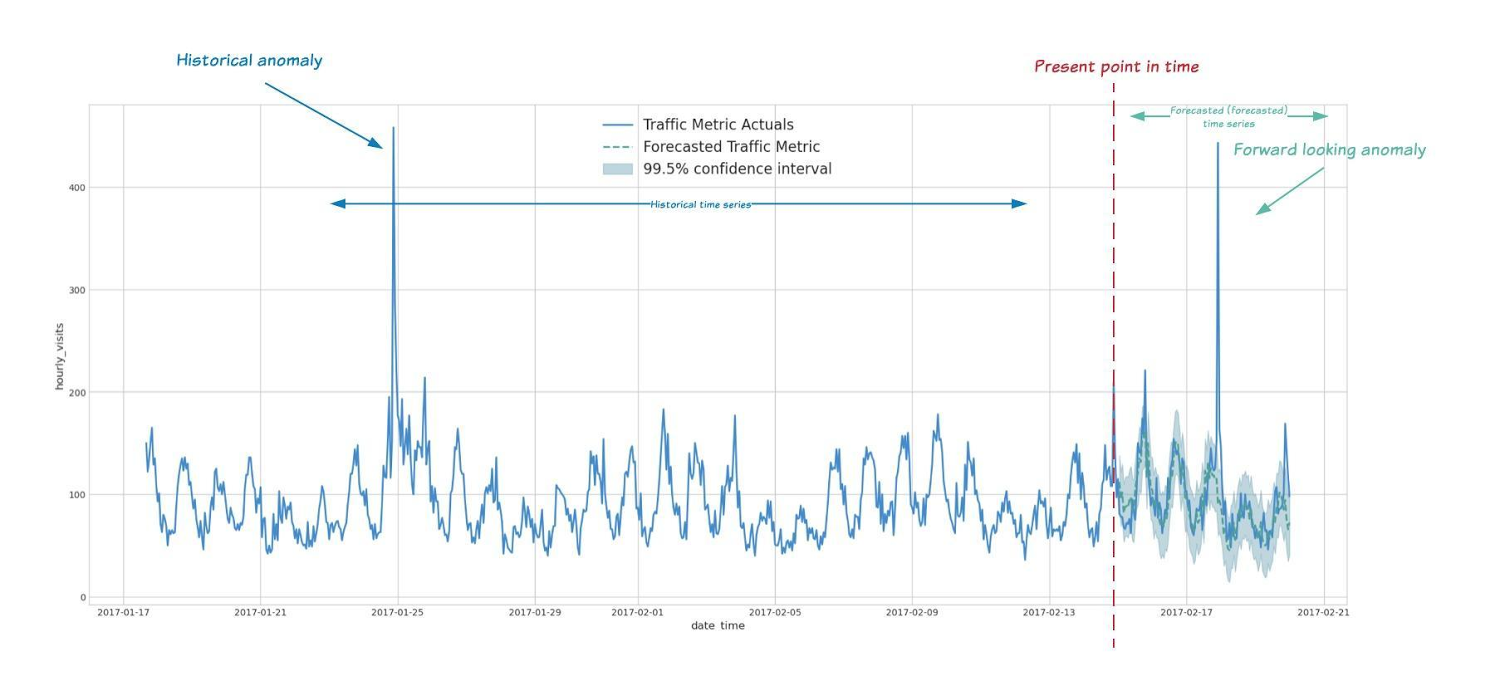
With ML.DETECT_ANOMALIES, you can now detect anomalies using ARIMA_PLUS time series models in the (historical) training data or in new input data. Here are some examples of when might you want to detect anomalies with time-series data:
Detecting anomalies in historical data:
- Cleaning up data for forecasting and modeling purposes, e.g. preprocessing historical time series before using them to train an ML model.
- When you have a large number of retail demand time series (thousands of products across hundreds of stores or zip codes), you may want to quickly identify which stores and product categories had anomalous sales patterns, and then perform a deeper analysis of why that was the case.
Forward looking anomaly detection:
- Detecting consumer behavior and pricing anomalies as early as possible: e.g. if traffic to a specific product page suddenly and unexpectedly spikes, it might be because of an error in the pricing process that leads to an unusually low price.
- When you have a large number of retail demand time series (thousands of products across hundreds of stores or zip codes), you would like to identify which stores and product categories had anomalous sales patterns based on your forecasts, so you can quickly respond to any unexpected spikes or dips.
How do you detect anomalies using ARIMA_PLUS? Begin by creating an ARIMA_PLUS time series model:
Language: SQL
CREATE OR REPLACE MODEL mydataset.my_arima_plus_modelOPTIONS(MODEL_TYPE='ARIMA_PLUS',TIME_SERIES_TIMESTAMP_COL='date',TIME_SERIES_DATA_COL='total_amount_sold',TIME_SERIES_ID_COL='item_name',HOLIDAY_REGION='US') ASSELECTdate,item_description AS item_name,SUM(bottles_sold) AS total_amount_soldFROM`bigquery-public-data.iowa_liquor_sales.sales`GROUP BYdate,item_nameHAVINGdate BETWEEN DATE('2016-01-04') AND DATE('2017-06-01')AND item_name IN ("Black Velvet", "Captain Morgan Spiced Rum","Hawkeye Vodka", "Five O'Clock Vodka", "Fireball Cinnamon Whiskey");
To detect anomalies in the training data, use ML.DETECT_ANOMALIES with the model obtained above:
Language: SQL
SELECT*FROMML.DETECT_ANOMALIES(MODEL `mydataset.my_arima_plus_model`,STRUCT(0.8 AS anomaly_prob_threshold));
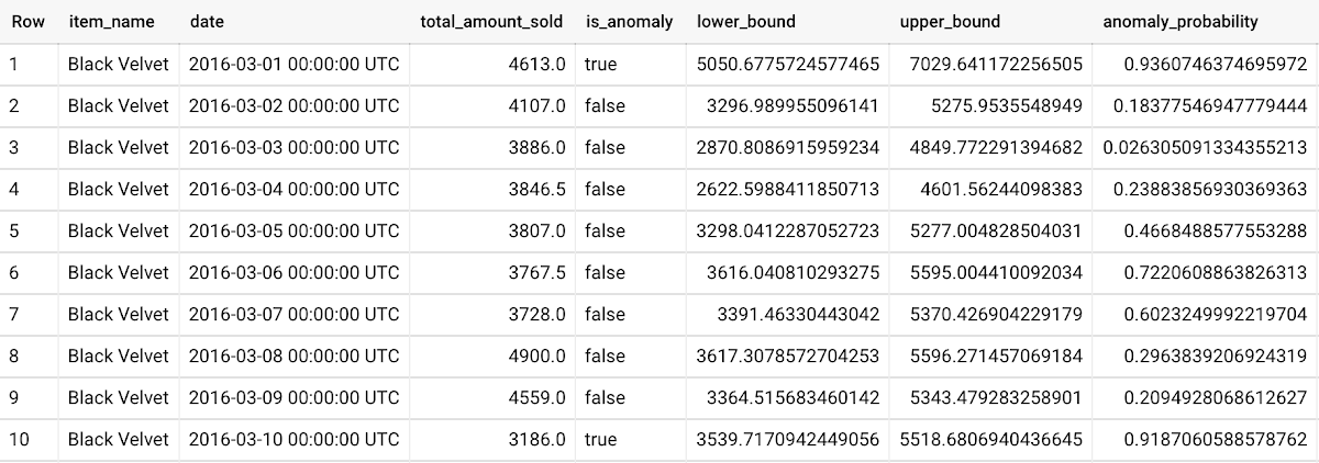
To detect anomalies in new data, use ML.DETECT_ANOMALIES and provide new data as input:
Language: SQL
WITHnew_data AS (SELECTdate,item_description AS item_name,SUM(bottles_sold) AS total_amount_soldFROM`bigquery-public-data.iowa_liquor_sales.sales`GROUP BYdate,item_nameHAVINGdate BETWEEN DATE('2017-06-02')AND DATE('2017-10-01')AND item_name IN ('Black Velvet','Captain Morgan Spiced Rum','Hawkeye Vodka',"Five O'Clock Vodka",'Fireball Cinnamon Whiskey') )SELECT*FROMML.DETECT_ANOMALIES(MODEL `mydataset.my_arima_plus_model`,STRUCT(0.8 AS anomaly_prob_threshold),(SELECT*FROMnew_data));
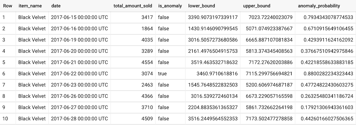
For more information on anomaly detection with ARIMA_PLUS time series models, please see the documentation here.
Thanks to the BigQuery ML team, especially Abhinav Khushraj, Abhishek Kashyap, Amir Hormati, Jerry Ye, Xi Cheng, Skander Hannachi, Steve Walker, and Stephanie Wang.
Time-series Model on Google Cloud Allows Better Transparency on Fishing and Marine Activities

4402
Of your peers have already read this article.
3:30 Minutes
The most insightful time you'll spend today!
Who would have known that today technology would enable us with the ability to use machine learning to track vessel activity, and make pattern inferences to help address IUU (illegal, unreported, and unregulated) fishing activities. What’s even more noteworthy is that we now have the computing power to share this information publicly in order to enable fair and sustainable use of our ocean.
An amazing group of humans at the nonprofit Global Fishing Watch took on this massive big data challenge and succeeded. You can immediately access their dynamic map on their website globalfishingwatch.org/map that is bringing greater transparency to fishing activity and supporting the creation and management of marine protected areas throughout the world.
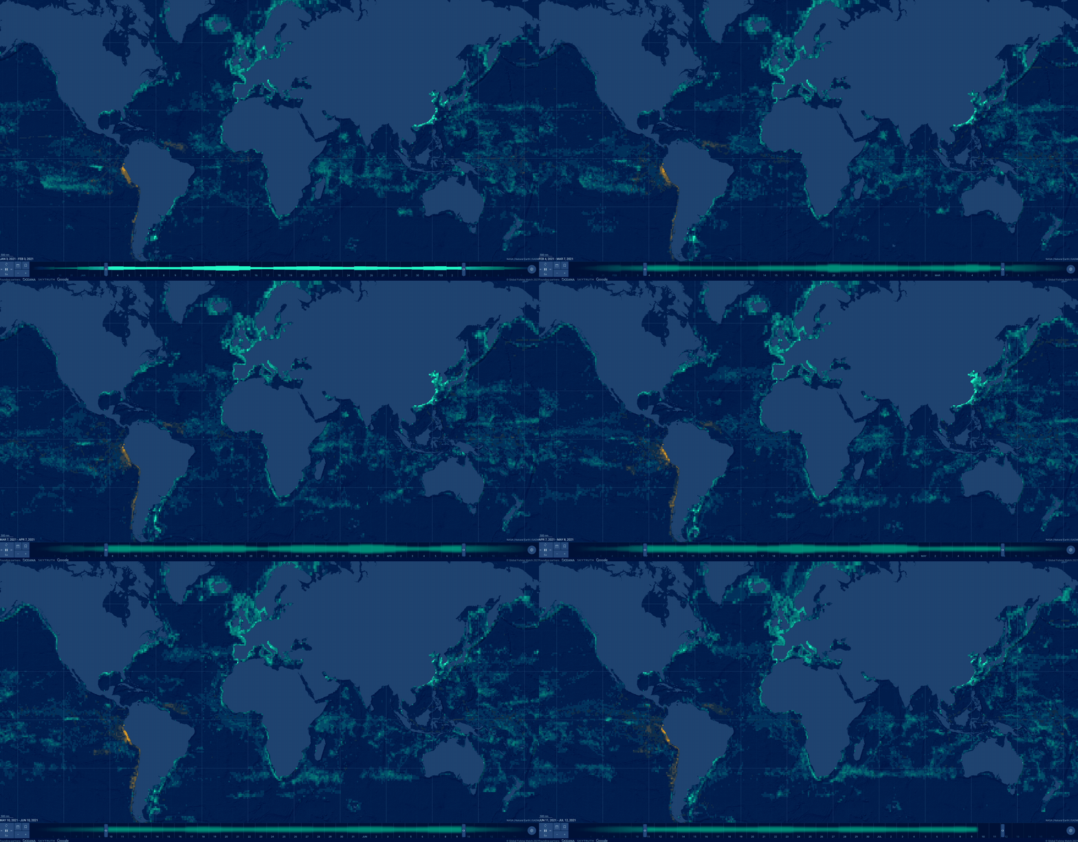
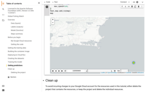
In our second episode of our People and Planet AI series we were inspired by their ML solution to this challenge, and we built a short video and sample with all the relevant code you need to get started with building a basic time-series classification model in Google Cloud, and visualize it in an interactive map.
Architecture
These are the components used to build a model for this sample:
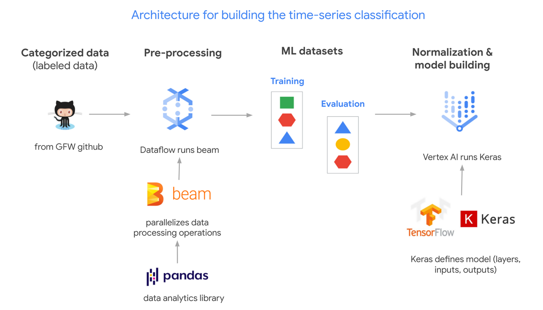
- Global Fishing Watch GitHub: where we got the data
- Apache Beam: (open source library) runs on Dataflow.
- Dataflow: (Google’s data processing service) creates 2 datasets; 1 for training a model and the other to evaluate its results.
- TensorflowKeras: (high level API library) used to define a machine learning model, which we then train in Vertex AI.
- Vertex AI: (a platform to build, deploy, and scale ML models) we train and output the model.
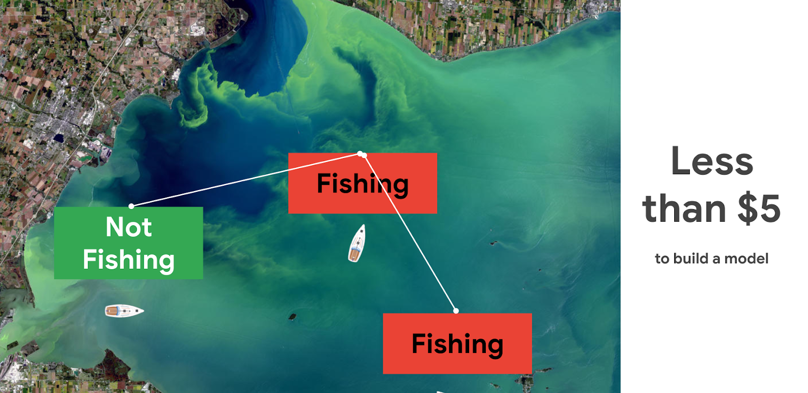
Pricing and steps
The total cost to run this solution was less than $5.
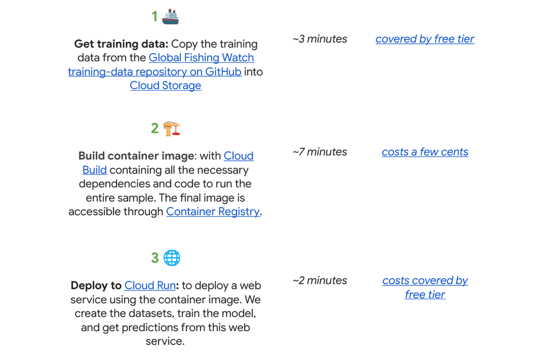
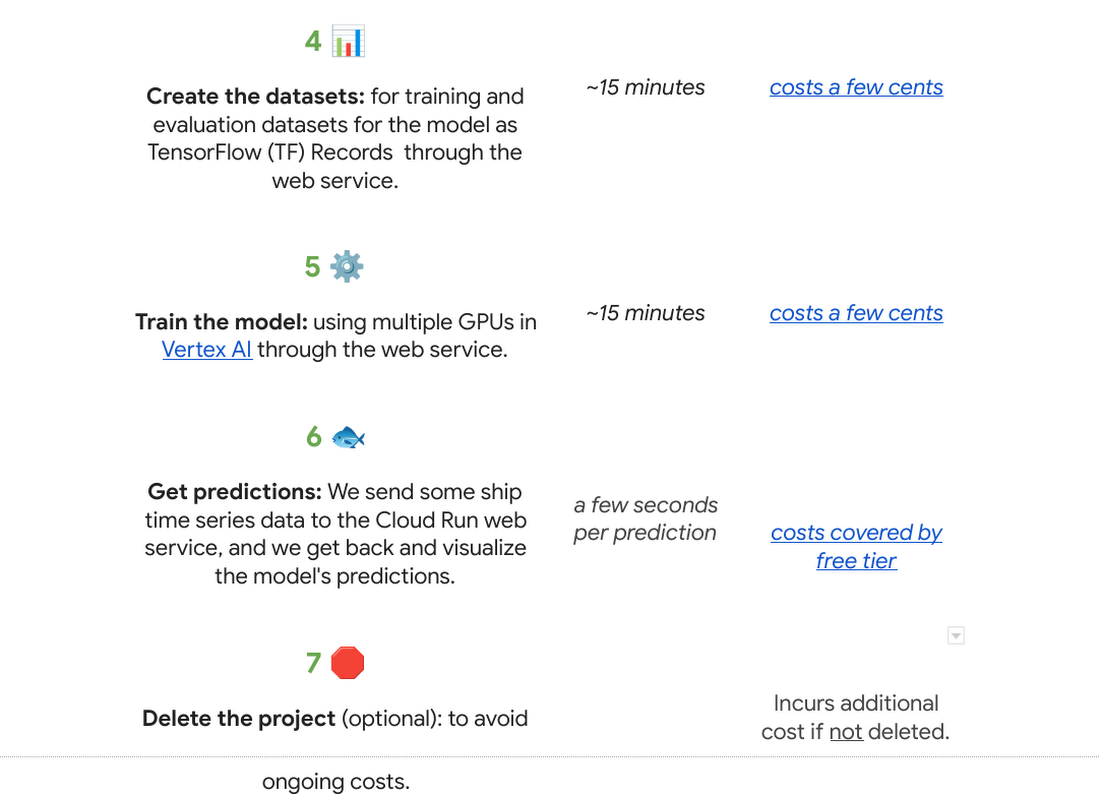
There are seven steps we went through with their approximate time and cost:
Why do we use a time series classification model?
Vessels in the ocean are constantly moving, which creates distinctive patterns from a satellite view.

We can train a model to recognize the shapes of a vessel’s trajectory. Large vessels are required to use the automatic identification system, or AIS. The GPS-like transponders regularly broadcast a vessel’s maritime mobile service identity, or MMSI, and other critical information to nearby ships, as well as to terrestrial and satellite receivers. While AIS is designed to prevent collisions and boost overall safety at sea, it has turned out to be an invaluable system for monitoring vessels and detecting suspicious fishing behavior globally.

One tricky part is that the MMSI data location signal (which includes a timestamp, latitude, longitude, distance from port, and more) is not emitted at regular intervals. AIS broadcast frequency changes with vessel speed (faster at higher speeds), and not all AIS messages that are broadcast are received – terrestrial receivers require line-of-sight, satellites must be overhead, and high vessel density can cause signal interference. For example, AIS messages might be received frequently as a vessel leaves the docks and operates near shore, then less frequently as they move further offshore until satellite reception improves. This is challenging for a machine learning model to interpret. There are too many gaps in the data, which makes it hard to predict.
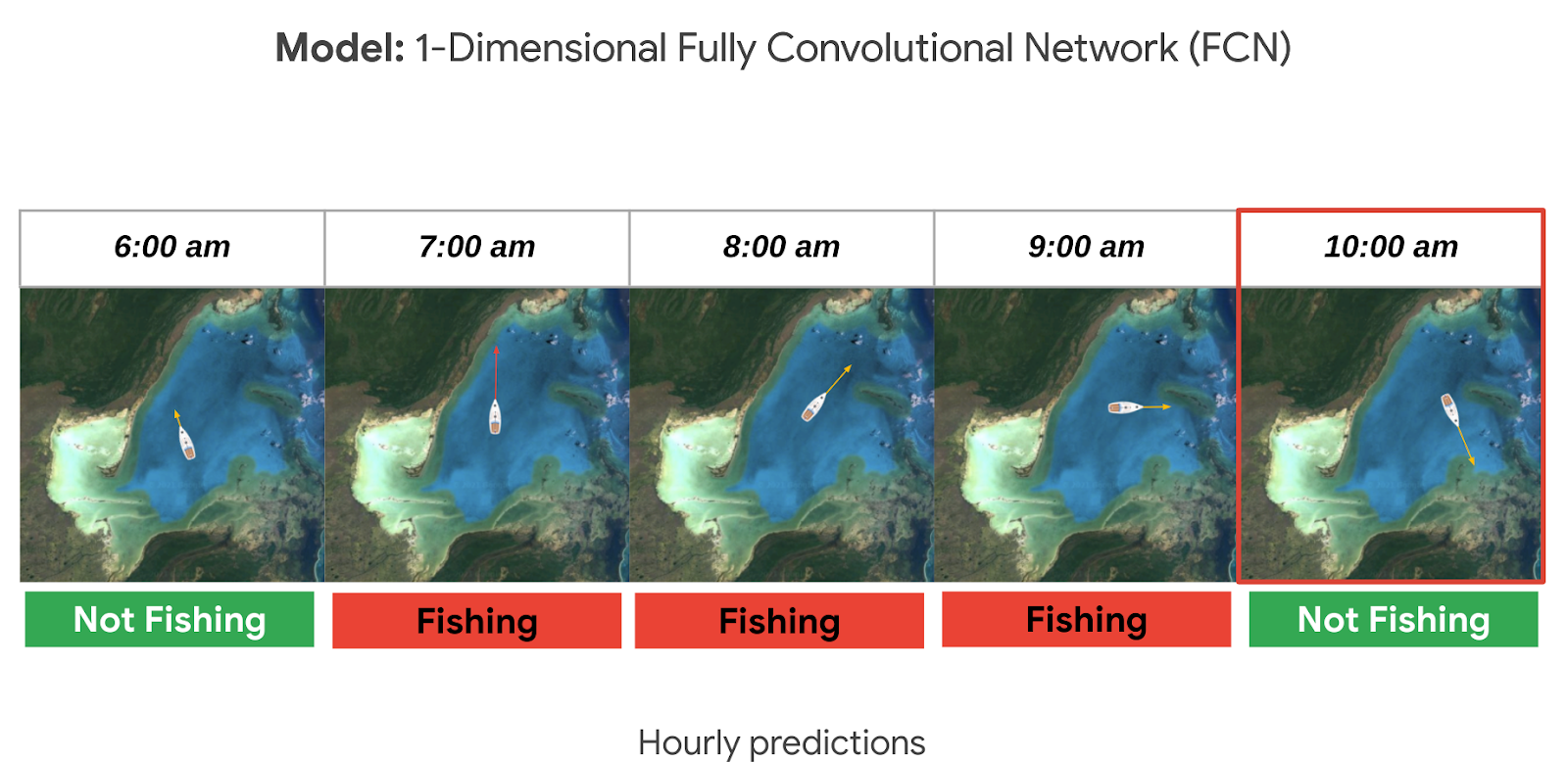
A way to solve this is to normalize the data and generate fixed-sized hourly windows. Then the model can predict if the vessel is fishing or not fishing for each hour.

It could be hard to know if a ship is fishing or not by just looking at its current position, speed, and direction. So we look at the data from the past as well, looking at the future could also be an option if we don’t need to do real time predictions. For this sample, it seemed reasonable to look 24 hours into the past to make a prediction. This means we need at least 25 hours of data to make a prediction for a single hour (24 hours in the past + 1 current hour). But we could predict longer time sequences as well. In general, to get hourly predictions, we need (n+24) hours of data.
Options to deploy and access the model
For this sample specifically we used Cloud Run to host the model as a web app so that other apps can call it to make predictions on an ongoing basis; this is our favorite in terms of pricing if you need to access your model from the internet over an extended period of time (charged per prediction request). You can also host it directly from Vertex AI where you trained and built the model, just note there is an hourly cost for using those VMs even if they are idle. If you do not need to access the model over the internet, you can make predictions locally or download the model onto a microcontroller if you have an IoT sensor strategy.

Want to go deeper?
If you found this project interesting and would like to dive deeper either into the specifics of the thought process behind each step of this solution or even run through the code in your own project (or test project); we invite you to check out our interactive sample hosted on Colab, which is a free Jupyter notebook. It serves as a guide with all the steps to run the sample, including visualizing the predictions on a dynamically moving map using an open source Python library called Folium.
There’s no prior experience required! Just click “open in Colab” which is linked at the bottom of GitHub.
You will need a Google Cloud Platform project. If you do not have a Google Cloud project you can create one with the free $300 Google Cloud credit, you just need to ensure you set up billing, and later delete the project after testing the desired sample.
🌏🌎🌍 We hope to inspire you to build other beautiful climate-related solutions.
Bit Capital Rolls Out a Digital Financial Solution in Under 3 Months and at 2/3 the Cost

5684
Of your peers have already read this article.
4:00 Minutes
The most insightful time you'll spend today!
In the past few years, a series of new technologies and regulatory changes has been transforming Brazil’s financial industry. The concept of blockchain added security and agility to financial transactions. The open banking system being deployed by the country’s Central Bank (BC) allows for platform integration and data sharing -with the user’s consent- between financial institutions. Recently, the launch of Pix, also by the BC, has shaken the market by creating a new payment method that is instant, free for individuals and 24/7.
Since 2018, the startup Bit Capital has been working on the development of 100%-digital financial solutions in the cloud to help its clients adapt to this new scenario in a convenient way, without the need to build an infrastructure for that or hiring different providers. Pix was not the exception.
In less than 3 months, the team was able to build and go live with a solution that can be used by both direct participants (i.e. those with banking licenses granted by BC) and indirect participants (i.e. companies depending on direct participants to offer payments on Pix) through Bit Capital’s platform.
Besides this differential, Pix and the startup’s other solutions are based on blockchain and Google Cloud’s cloud, ensuring greater security, scalability and availability for customers and allowing for an easy integration between Bit Capital’s platform’s solutions and those from other companies.
“Now we have a platform with an API and various microsservices, allowing clients to connect and develop their own financial product without having to start from scratch.”
—Francesco Miolo, CFO, Bit Capital
A robust structure to handle Pix’s high demand
Bit Capital was established with a certain urgency to develop its platform. The idea was well-developed and customers were interested. The fast deployment of Google Cloud’s tools was one of the main factors that attracted the company to use it as a basis for its infrastructure.
“We managed to deliver everything we have today in Google Cloud with a small team. That was another challenge: being able to grow with a few people,” says Juliano Souza, the startup’s head of IT infrastructure. “We sought other cloud partners, but they had a steep curve. We chose Google Cloud because we needed quick, quality scaling.”
The same thing happened when they built the solution for Pix, despite the specific challenges involved. The BC had performance requirements that led the company to spend some time experimenting until they reached the best suite of tools to meet those requirements. The startup wanted to create a unique architecture that could help both large and small customers and be integrated to the platform’s other microservices.
With the support from Google Cloud’s team to answer doubts and make the best decisions, the solution was built in a few months, at a cost about two-thirds lower than other providers.
The solution’s architecture is based on apps running in Docker in Google Kubernetes Engine (GKE), with interconnected microservices. The blockchain system runs on Compute Engine, its rows are managed in Pub/Sub and Dataflow, and persistent data, in Cloud SQL. Cloud Interconnect is used for the connection with BC. Cloud KMS and Secrets Management store the company’s pre-credentials. All of this is supported by Cloud Load Balancing for load balancing and autoscaling.
According to the team, GKE was essential for the solution’s success. Using infrastructure as code in the tool made uploading of a group of microservices significantly easier. Developers are able to help set up this environment, which has helped spread the DevOps culture in the team. Besides orchestrating and integrating apps, GKE also provides an elastic structure to handle demand peaks and visibility to monitor internal components.
“Google Kubernetes Engine was the only way to ensure availability, observability and elasticity for all clients, whether small, middle-sized or large.”
—Juliano Souza, Head of IT Infrastructure, Bit Capital
Nowadays, the solution’s environment has 20 clusters with over 1,500 pods – 250GB in data per month, providing a robust structure to support a service involving periods of intense demand such as Black Friday.
Ease to monitor, fix and improve
Just 10 days after Pix’s official launch date, the company had its first test: Black Friday. This allowed a major e-commerce customer to test the scale and see the success of the architecture that had been built. “It worked great regarding what the cloud could deliver. And we found what we needed to fix very quickly. Operations [formerly Stackdriver], in particular Cloud Trace, showed us clearly what needed to be done to improve performance,” Souza explains.
Using Operations added reliability by putting deliveries into production. Checking Cloud Trace to see if there were any performance issues and the exact point where they were happening became routine for Bit Capital’s developers. Google Cloud’s security tools and Google Safety Center provided the resources needed to monitor and secure the environment, with automatic data encryption at rest and in transit.
“Google Cloud has security as a premise. When we upload any kind of component, like a database or a virtual machine, the drive is encrypted by default. With other providers, you must specify that you want it encrypted.
”—Juliano Souza, Head of IT Infrastructure, Bit Capital
The easy service monitoring and management accelerates product and technology development because the team no longer needs to worry about infrastructure. Automated management allows professionals to spend more time on new projects and the company’s business. Also, the deployment of services in a Google Cloud multi-region impacts on customer experience, providing high availability for their solutions.
In the coming months, Bit Capital aims to ramp up service usage and the creation of new projects in Google Cloud by adding more customers to Pix’s solution and Banking as a Service (BaaS) solutions. Anthos will be incorporated to the tool suite to make it easier to connect apps with the customers’ on-prem environments. And the deployment of open banking has the potential to be a business driver for the company.
“We joke that we’re already doing open banking, because we have various connections with different providers, which allows us to offer an integrated solution,” says Francesco Miolo, the startup’s CFO. “With the arrival of the new regulations, something we are waiting for since we started out, we will be able, through our platform, to take our customers to the open finance ecosystem, enabling the development of disruptive business models.”
More Relevant Stories for Your Company
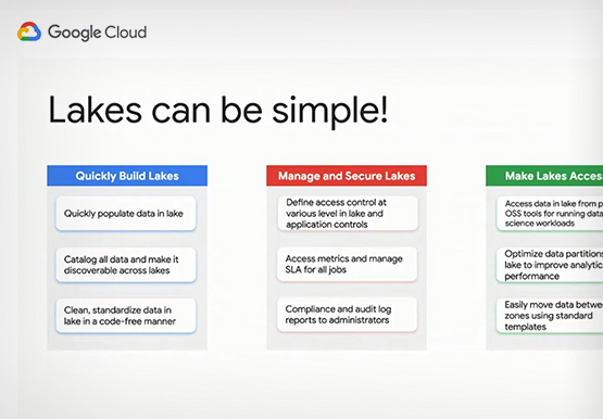
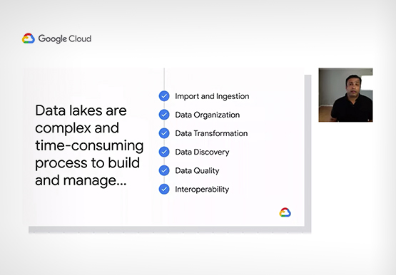
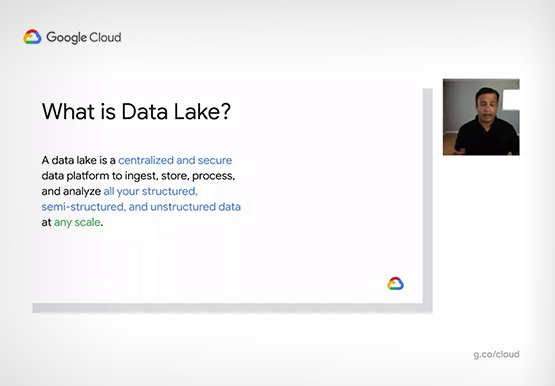

Building Data Lakes on Google Cloud
A data lake is a centralized and a secure data platform for ingesting, storing, processing, and analyzing all your data--structured semi-structured and unstructured data--at scale. “When we work with our customers we find out that the traditional approach for building data lakes, where you bring data from different sources and

An Expert’s Opinion on What Early-stage Startups Must Know
As lead for analytics and AI solutions at Google Cloud, my team works with startups building on Google Cloud. This puts us in the fortunate position to learn from founders and engineers about how early-stage startups’ investments can either constrain them or position them for success, even at the seed

A Pre-ML Checklist That Will Save You Hours of Work
One of the toughest challenges for data scientists, and big data engineers is gathering, preparing, and transforming data, and creating data pipelines. Gathering data for a machine learning or big data initiative can be hard work. The mere act of getting it all together can leave data teams so excited

How Machine Learning Can Cut Support Ticket Resolution Time By Over 80%
Sure, machine learning is becoming a business imperative, but how does it work in practice—and what are the benefits for IT managers? That’s the subject of a new step-by-step guide to solving business and IT problems with artificial intelligence and ML, based on insights gathered by IDG Research Services. Its
