





Unification of Dataplex and Data Catalog: A Full Spectrum of Data Governance and Data Management at Scale

2967
Of your peers have already read this article.
2:30 Minutes
The most insightful time you'll spend today!
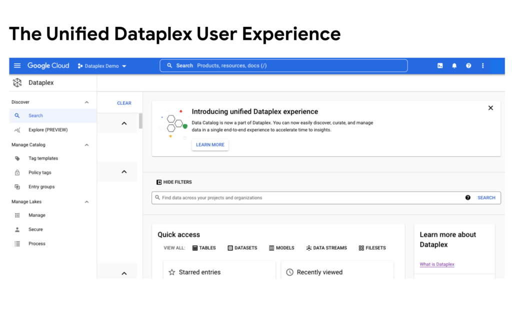
Today, we are excited to announce that Google Cloud Data Catalog will be unified with Dataplex into a single user interface. With this unification, customers have a unified experience to search and discover their data, enrich it with relevant business information, organize it by logical data domains, and centrally govern and monitor their distributed data with built-in data intelligence and automation capabilities. Customers now have access to an integrated metadata platform that connects technical and operational metadata with business metadata, and then uses this augmented and active metadata to drive intelligent Data management and governance got easier the unification of Dataplex and Data Catalog
The enterprise data landscape is becoming increasingly diverse and distributed with data across multiple storage systems, each having its own way of handling metadata, security, and governance. This creates a tremendous amount of operational complexity, and thus, generates strong market demand for a metadata platform that can power consistent operations across distributed data.
Dataple provides a data fabric to automate data management, governance, discovery, and exploration across distributed data at scale. With Dataplex, enterprises can easily arrange their data into data domains, delegate ownership, usage, and sharing of data to data owners who have the right business context, while still maintaining a single pane of glass to consistently monitor and govern data across various data domains in their organization.
Prior to this unification, data owners, stewards and governors had to use two different interfaces – Dataplex to organize, manage, and govern their data, and Data Catalog to discover, understand, and enrich their data. Now with this unification, we are creating a single coherent user experience where customers can now automatically discover and catalog all the data they own, understand data lineage, check for data quality, augment with business knowledge, organize data into domains, and then use that combined metadata to power data management. Together we provide an integrated experience that serves the full spectrum of data governance needs in an organization, enabling data management at scale.
“With Data Catalog now being part of Dataplex, we get a unified, simplified, and streamlined experience to effectively discover and govern our data, which enables team productivity and analytics agility for our organization. We can now use a single experience to search and discover data with relevant business context, organize and govern this data based on business domains, and enable access to trusted data for analytics and data science – all within the same platform.” said Elton Martins, Senior Director of Data Engineering at Loblaw Companies Limited.
Getting started
Existing Data Catalog and Dataplex customers and new customers can now start using Dataplex for metadata discovery, management and governance. Please note that while the user experience interface is unified via this release, all existing APIs and feature functionalities of both products will continue to work as before. To learn more, please refer to technical documentations or contact the Google Cloud sales team.
BigQuery Reference Guide: Understanding Tables within and Routine for Data Transformation

3684
Of your peers have already read this article.
3:00 Minutes
The most insightful time you'll spend today!
Last week in our BigQuery Reference Guide series, we spoke about the BigQuery resource hierarchy – specifically digging into project and dataset structures. This week, we’re going one level deeper and talking through some of the resources within datasets. In this post, we’ll talk through the different types of tables available inside of BigQuery, and how to leverage routines for data transformation. Like last time, we’ll link out to the documentation so you can learn more about using these resources in practice.
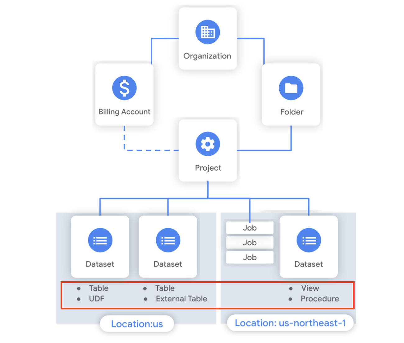
What is a table?
A BigQuery table is a resource that lives inside a dataset. It contains individual records organized into rows, with each record composed of columns (also called fields) where a specified data type is enforced. BigQuery supports numerous different data types including GEOGRAPHY for geospatial data, STRUCT and ARRAY for more complex data, and new parameterized data types to add specific constraints like the number of characters in a string.
Data access can also be controlled at the table, row and column levels; more details on data governance will be covered later in the series. Metadata, such as descriptions and labels, can be used for surfacing information to end users and as tags for monitoring. You can create and manage a table directly in the UI, through the API / Client SDKs or in a SQL query using a DDL statement.
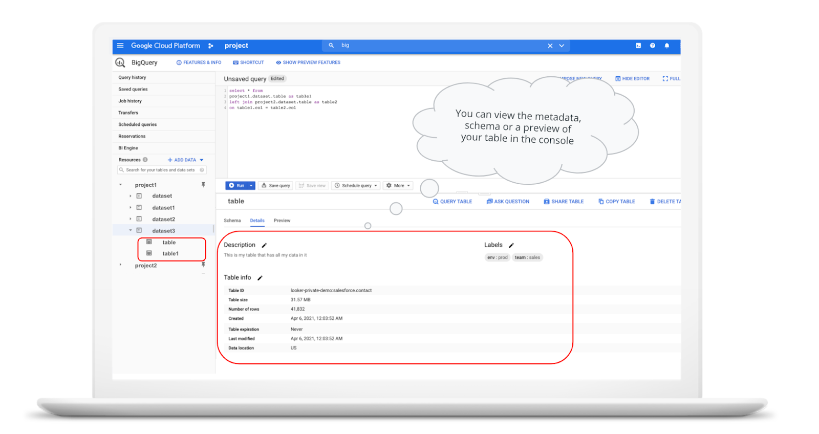
bq show \--schema \--format=prettyjson \project1:dataset3.table
Managed and external tables
Managed tables are tables that are backed by native BigQuery storage, which has many benefits that improve query performance including support for partitions and clusters. We’ll cover more details on BigQuery storage later in this series. Another advantage of using a managed table is that BigQuery allows you to use time travel to access data from any point within the last seven days and query data that was updated, expired or deleted. And now you can even create a snapshot of your table, to preserve its contents at a given time.
# create a snapshot of transactions in the library_backup dataset as of one hour agoCREATE SNAPSHOT TABLElibrary_backup.salesCLONE retail.transactionsFOR SYSTEM_TIME AS OF TIMESTAMP_SUB(CURRENT_TIMESTAMP(), INTERVAL 1 HOUR);
While managed tables store data inside BigQuery storage, external tables are backed by storage external to BigQuery. BigQuery currently supports creating an external table from Cloud Storage, Cloud Bigtable and Google Drive. Besides an external table, you can create a connection to Cloud SQL, which is somewhat analogous to an external dataset. Here, you can leverage federated queries to send a query that executes in Cloud SQL but returns the results to be used within BigQuery.
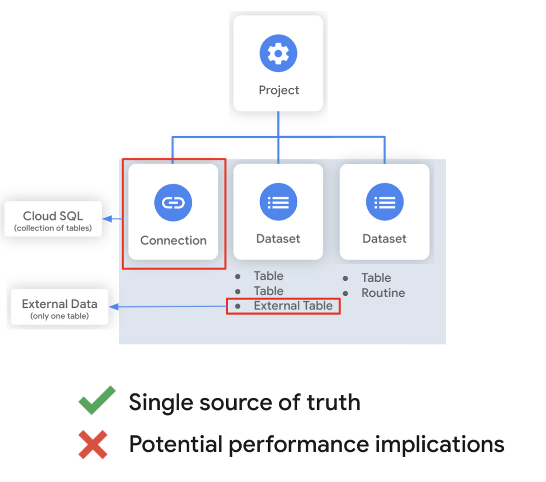
Using external tables or federated queries may result in queries that aren’t as fast as if the data had been stored in BigQuery itself. However, they can be useful for some data transformation patterns – for example, you may want to schedule a DDL/DML query that hydrates a managed table using a federated query, which selects and transforms data from Cloud SQL. An external table might also be useful for multi-consumer workflows where BQ storage isn’t the source of truth. Like, if you have a dataproc cluster accessing data in a Cloud Storage bucket that you’re not quite ready to port into BigQuery (although I do recommend taking a look at our connector if you need some convincing). You can learn more about querying external data in this video.
Logical and materialized views
In BigQuery, you can create a virtual table with a logical view or a materialized view. With logical views, BigQuery will execute the SQL statement to create the view at run time, it will not save the result anywhere. Additionally, you can grant users access to an authorized view to share query results without giving them access to the underlying tables.
# create a view that aggregates daily sales from a retail transaction tableCREATE VIEW retail.daily_sales as (SELECT date(t.transaction_timestamp) as date, sum(li.sale_price) as total_salesFROM retail.transaction_detail as tLEFT JOIN UNNEST(t.line_items) as liGROUP BY 1)
On the other hand, materialized views are re-computed in the background when the base data changes. No user action is required – they are always fresh! Better yet, if a query, or part of a query, against the source table can be resolved by querying the materialized view, BigQuery will reroute for improved performance. However, materialized views use a restricted SQL syntax and a limited set of aggregation functions. You can find details on limitations here.
# create a materialized view that aggregates daily salesCREATE MATERIALIZED VIEW retail.daily_sales as (SELECT date(t.transaction_timestamp) as date, sum(li.sale_price) as total_salesFROM retail.transaction_detail as tLEFT JOIN UNNEST(t.line_items) as liGROUP BY 1)
Temporary and cached results tables
Aside from the tables we’ve mentioned so far, you can also create a temporary managed table using the TEMP or TEMPORARY keyword. This table is saved in BigQuery storage and can be referenced for the duration of the script. Temporary tables can be a good alternative to WITH clauses because the defining query is only executed once as opposed to being inlined every place the alias is referenced.
| Original code | Optimized |
| with a as ( select …),b as ( select … from a …),c as ( select … from a …)select b.dim1, c.dim2from b, c; | create temp table a asselect …; with b as ( select … from a …),c as ( select … from a …)select b.dim1, c.dim2from b, c; |
It’s also important to mention that BigQuery writes all query results to a table – one either explicitly identified by the user or to a cached results table. Temporary, cached results tables are maintained per-user, per-project. There are no storage costs for temporary tables.
User defined functions & procedures
In BigQuery, a routine is either a user defined function (UDF) or a procedure. Routines allow you to re-use logic and handle your data in a unique way. A UDF is a function that is created using either SQL or Javascript, it takes arguments as input and returns a single value as an output. UDFs are often used for cleaning or re-formatting data. For example, extracting parameters from a URL string, restructuring nested data, or cleaning up strings:
# UDF to clean up string valuesCREATE OR REPLACE FUNCTIONmy_dataset.cleanse_string_test (text STRING)RETURNS STRINGAS (REGEXP_REPLACE(LOWER(TRIM(text)), '[^a-zA-Z0-9 ]+', ''));
We even have a community driven open-source repository of BigQuery UDFs! Just like logical views, you can create an authorized UDF that protects aspects of the underlying data. For more details on UDFs checkout our video here. You might also want to take a look at table functions – a preview feature where you can create a SQL UDF that returns a table instead of a scalar value.
Procedures, on the other hand, are blocks of SQL statements that can be called from other queries. Unlike UDFs, stored procedures can return multiple values or no values – which means you can run them to create or modify tables. In BigQuery, you can also leverage scripting capabilities within procedures to control execution flow with IF and WHILE statements. Plus, you can call your UDFs within your procedure! These aspects make procedures great for extract-load-transform (ELT) driven workflows.
# Procedure to create daily sales rollup, starting from startDate until endDateCREATE OR REPLACE PROCEDURE my_dataset.sum_sales(startDate STRING, endDate STRING)BEGINCREATE OR REPLACE TABLE retail.sales_resultAS (SELECTdate(t.transaction_timestamp) as date,sum(li.sale_price) as total_salesFROM retail.transaction_detail as tLEFT JOIN UNNEST(t.line_items) as liWHERE transaction_timestamp >= TIMESTAMP(startDate) AND transaction_timestamp <= TIMESTAMP(endDate)GROUP BY 1);END;CALL retail.sum_sales('2020-08-01', '2020-01-20');
To ensure consistent analytics across your organization, I recommend that you create a library dataset to house UDFs and procedures. You can easily grant everyone in your organization the BigQuery Data Viewer role to the library dataset so that all analysts use consistent and up-to-date logic in their queries.
Stay tuned!
We hope this gave you an understanding of how to leverage some of the different resources inside of a BigQuery dataset, and to help you make decisions like using native versus external storage, logical versus materialized views, and user defined functions or procedures.
Next up we’ll be talking about workload management in BigQuery by taking a look at jobs and the reservation model. Be sure to keep an eye out for more in this series by following me on LinkedIn and Twitter, and subscribing to our Youtube channel.
Soundtrack Your Brand: Delivering Sound That Stands Out From the Crowd with BigQuery

2841
Of your peers have already read this article.
6:00 Minutes
The most insightful time you'll spend today!
Editor’s note: Soundtrack Your Brand is an award-winning streaming service with the world’s largest licensed music catalog built just for businesses, backed by Spotify. Today, we hear how BigQuery has been a foundational component in helping them transform big data into music.
Soundtrack Your Brand is a music company at its heart, but big data is our soul. Playing the right music at the right time has a huge influence on the emotions a brand inspires, the overall customer experience, and sales. We have a catalog of over 58 million songs and their associated metadata from our music providers and a vast amount of user data that helps us deliver personalized recommendations, curate playlists and stations, and even generate listening schedules. As an example, through our Schedules feature our customers can set up what to play during the week. Taking that one step further, we provide suggestions on what to use in different time slots and recommend entire schedules.
Using BigQuery, we built a data lake to empower our employees to access all this content and metadata in a structured way. Ensuring that our data is easily discoverable and accessible allows us to build any type of analytics or machine learning (ML) use case and run queries reliably and consistently across the complete data set. Today, our users are benefiting from this advanced analytics through the personalized recommendations we offer across our core features: Home, Search, Playlists, Stations, and Schedules.
Fine-tuning developer productivity
The biggest business value that comes from BigQuery is how much it speeds up our development capabilities and allows us to ship features faster. In the past 3 years, we have built more than 150 pipelines and more than 30 new APIs within our ML and data teams that total about 10 people. That is an impressive rate of a new pipeline every week and a new API every month. With everything in BigQuery, it’s easy to simply write SQL and have it be orchestrated within a CI/CD toolchain to automate our data processing pipelines. An in-house tool built as a github template, in many ways very similar to Dataform, helps us build very complex ETL processes in minutes, significantly reducing the time spent on data wrangling.
BigQuery acts as a cornerstone for our entire data ecosystem, a place to anchor all our data and be our single source of truth. This single source of truth has expanded the limits of what we can do with our data. Most of our pipelines start from a data lake, or end at a data lake, increasing re-usability of data and collaboration. For example, one of our interns built an entire churn prediction pipeline in a couple of days on top of existing tables that are produced daily. Nearly a year later, this pipeline is still running without failure largely due to its simplicity. The pipeline is BigQuery queries chained together into a BigQuery ML model running on a schedule with Kubeflow Pipelines.
Once we made BigQuery the anchor for our data operations, we discovered we could apply it to use cases that you might not expect, such as maintaining our configurations or supporting our content management system. For instance, we created a Google Sheet where our music experts are able to correct genre classification mistakes for songs by simply adding a row to a Google Sheet. Instead of hours or days to create a bespoke tool, we were able to set everything up in a few minutes.
BigQuery’s ability to consume Excel spreadsheets allows business users who play key roles in improving our recommendations engine and curating our music, such as our content managers and DJs, to contribute to the data pipeline.
Another example is our use of BigQuery as an index for some of our large Cloud Storage buckets. By using cloud functions to subscribe to read/write events for a bucket, and writing those events to partitioned tables, our pipelines can easily and in a natural way quickly search and access files, such as downloading and processing the audio of new track releases. We also make use of Log Events when a table is added to a dataset to trigger pipelines that process data on demand, such as JSON/CSV files from some of our data providers that are newly imported into BQ. Being the place for all file integration and processing, BQ allows new data to be quickly available to our entire data ecosystem in a timely and cost effective manner while allowing for data retention, ETL, ACL and easy introspection.
BigQuery makes everything simple. We can make a quick partitioned table and run queries that use thousands of CPU hours to sift through a massive volume of data in seconds — and only pay a few dollars for the service. The result? Very quick, cost-effective ETL pipelines.
In addition, centralizing all of our data in BigQuery makes it possible to easily establish connections between pipelines providing developers with a clear understanding of what specific type of data a pipeline will produce. If a developer wants a different outcome, she can copy the github template and change some settings to create a new, independent pipeline.
Another benefit is that developers don’t have to coordinate schedules or sync with each other’s pipelines: they just need to know that a table that is updated daily exists and can be relied on as a data source for an application. Each developer can progress their work independently without worrying about interfering with other developers’ use of the platform.
Making iteration our forte
Out of the box, BigQuery met and exceeded our performance expectations, but ML performance was the area that really took us by surprise. Suddenly, we found ourselves going through millions of rows in a few seconds, where the previous method might have taken an hour. This performance boost ultimately led to us improving our artist clustering workload from more than 24 hours on a job running 100 CPU workers to 10 minutes on a BigQuery pipeline running inference queries in a loop until convergence. This more than 140x performance improvement also came at 3% of the cost.
Currently we have more than 100 Neural Network ML models being trained and run regularly in batch in BQML. This setup has become our favorite method for both fast prototyping and creating production ready models. Not only is it fast and easy to hypertune in BQML, but our benchmarks show comparable performance metrics to using our own Tensorflow code. We now use Tensorflow sparingly. Differences in input data can have an even greater impact on the experience of the end user than individual tweaks to the models.
BigQuery’s performance makes it easy to iterate with the domain experts who help shape our recommendations engine or who are concerned about churn, as we are able to show them the outcome on our recommendations from changes to input data in real-time. One of our favorite things to do is to build a Data Studio report that has the ML.predict query as part of its data source query. This report shows examples of good/bad predictions in the report along with bias/variance summaries and a series of drop-downs, thresholds and toggles to control the input features and the output threshold. We give that report to our team of domain experts to help manually tune the models, putting the model tuning right in the hands of the domain experts. Having humans in the loop has become trivial for our team. In addition to fast iteration, the BigQuery ML approach is also very low maintenance. You don’t need to write a lot of Python or Scala code or maintain and update multiple frameworks—everything can be written as SQL queries run against the data store.
Helping brands to beat the band—and the competition
BigQuery has allowed us to establish a single source of truth for our company that our developers and domain experts can build on to create new and innovative applications that help our customers find the sound that fits their brand.
Instead of cobbling together data from arbitrary sources, our developers now always start with a data set from BigQuery and build forward. This guarantees the stability of our data pipeline and makes it possible to build outward into new applications with confidence. Moreover, the performance of BigQuery means domain experts can interact with the analytics and applications that developers create more easily and see the results of their recommended improvements to ML models or data inputs quickly. This rapid iteration drives better business results, keeps our developers and domain experts aligned, and ensures Soundtrack Your Brand keeps delivering sound that stands out from the crowd.
Home Depot’s Interconnected Retail Experience by Virtue of Google Cloud Migration for SAP Applications

8279
Of your peers have already read this article.
1:30 Minutes
The most insightful time you'll spend today!
With nearly 2,300 stores, The Home Depot is the world’s largest home-improvement chain — a brand that professional contractors and DIYers alike have come to depend on. The home improvement industry continues to experience unprecedented demand and dramatic increases in online ordering accompanied by expanding consumer expectations for things like curbside pickup and same day delivery. The Home Depot’s decision to migrate to cloud-based infrastructure, including the migration of the company’s SAP applications on Google Cloud which began in 2017, has set it up for success in an increasingly digital world, and helped the company adapt to changing market conditions quickly.
Interconnected retail at scale
Building on a strong customer-first philosophy, The Home Depot aims to create what it calls interconnected retail—allowing customers to shop however, whenever, and wherever they want. “So many companies are focused on omni-channel retail,” explains Sam Moses, Vice President of Corporate Systems. “At The Home Depot, we wanted to take it to the next level. Interconnected retail puts the customer at the center of everything and enables them to shop in store, online, or both. Customers can begin a transaction online and continue in-store, or vice-versa.”
To support this strategy, the company’s SAP environment needed to be more agile. Running everything on-premises, from central finance to POS systems, meant that The Home Depot’s IT teams experienced redundancy and repetitive, manual processes. Their data warehouse needed an upgrade to process and analyze growing and increasingly diverse data sets. The Home Depot chose to migrate its SAP environment to Google Cloud to support both the velocity and scale needed for the business as well as critical analytics capabilities needed for its bold digital initiatives. “We chose Google Cloud to support our SAP implementation. Our decision had a lot to do with the relationship between Google Cloud and SAP and also for the applications and services that are offered by Google Cloud, like BigQuery, which are helping to enable data and analytics within our organization,” Moses explains.
After migrating its SAP applications—including S/4HANA, its customer activity repository (CAR), general ledger, e-commerce system, enterprise data warehouse and more to Google Cloud, the company now has the speed, scale and flexibility to tackle enormous spikes in the business, all while staying fully available for their customers. Additionally, The Home Depot was able to transform its financial systems and make them more agile to deliver critical information across multiple business functions in real time.
Maximizing data insights to support customer experiences
By migrating to Google Cloud, The Home Depot is leveraging Google Cloud analytics to build the industry’s most efficient supply chain including more robust demand forecasting, supplier lead times, estimated delivery times and more, all while maintaining better security than before. “We experienced unprecedented change in our customers’ behavior and their buying patterns, which puts a lot of pressure on our supply chain,” explains Moses. “So having the ability to leverage data and analytics gives us insights to know exactly what it is that our customers need.”
The company’s analysts now use BigQuery ML for machine learning directly against the company’s BigQuery data and use AutoML to determine the best model for predictions. The Home Depot’s engineers have also adapted BigQuery to monitor, analyze, and act on application performance data across all its stores and warehouses in real time—capabilities that were not as seamless in the on-premises environment.
With hundreds of projects on Google Cloud, The Home Depot’s cloud journey is well on track, but the company is always looking to the future. “As our customers’ needs have continued to evolve, and as technology has continued to evolve, our relationship with Google will continue to advance — to be able to innovate together, to be able to find new solutions together, to better serve our customers.”
Learn more about how The Home Depot is renovating its retail operation with SAP on Google Cloud.
Experts’ Guideline for Personalizing Platforms with the Right Recommendation System on Google Cloud

5012
Of your peers have already read this article.
5:00 Minutes
The most insightful time you'll spend today!
Over the past two decades, consumers have become accustomed to receiving personalized recommendations in all facets of their online life. Whether that be recommended products while shopping on Amazon, a curated list of apps in the Google Play store, or relevant videos to watch next on YouTube. In fact, in a Verge article “How YouTube perfected the feed: Google Brain gave YouTube new life,” the Google Brain team reveals how their recommendation engine has impacted the platform with “more than 70 percent of the time people spend watching videos on the site being driven by YouTube’s algorithmic recommendations” thereby increasing time spent on the platform by 20X in three years.
It’s become clear that personalized recommendations are no longer a differentiator for an organization but rather something consumers have come to expect in their day-to-day experiences online. So what should you do if you are behind the curve and want to get started or simply want to improve upon what you already have? While there are all sorts of techniques, from content-based systems to deep learning methods, our goal in this recommender-focused blog series is to demystify three available approaches to building recommendation systems on Google Cloud: Matrix Factorization in BigQuery Machine Learning (BQML), Recommendations AI, and deep retrieval techniques available via the Two-Tower built-in algorithm.
One of these approaches can be used to meet you where you are in your personalization journey, no matter if you are just starting or if you are well into it. This first blog post will introduce our three approaches and when to use them.
What is Matrix Factorization and how does it work?
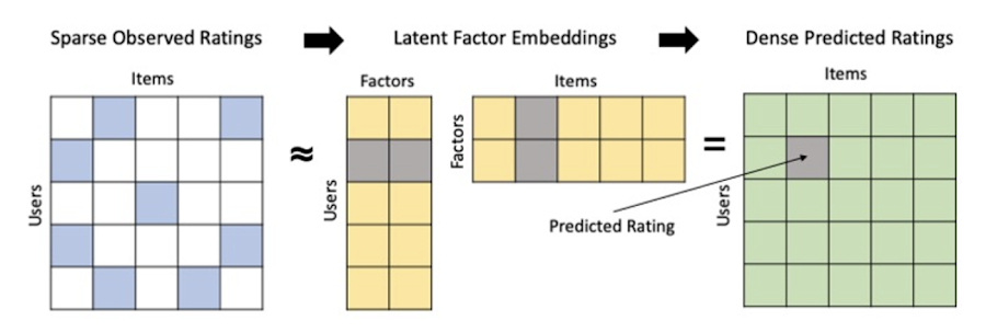
Collaborative filtering is a foundational model for building a recommendation system as the input dataset is simple and the embeddings are learned for you. How does Matrix factorization fit into the mix you might be wondering? Matrix factorization is simply the model that applies collaborative filtering. BQML enables users to create and execute a matrix factorization model by using standard SQL directly in the data warehouse.
Collaborative filtering begins by creating an interaction matrix. The interaction matrix represents users as a row and items as columns in your dataset. This interaction matrix often is sparse in nature as not all users will have interacted with many items in your catalog. This is where embeddings come into play. Generating embeddings for users and items not only allows you to collapse many sparse features into a lower dimensional space but they also allow you to derive a similarity measure so that similar users/items fall nearby in the embedding space. These similarity measures are key as collaborative filtering uses similarities between users and items to make the end recommendations. The underlying assumption being that similar users will like similar items whether that be movies or handbags.
What’s required to get started?
To train a matrix factorization model you need a table that includes three input columns: user(s), item(s), and an implicit or explicit feedback variable (e.g., ratings is an example of explicit feedback). With the base input dataset in place, you can then easily run your model in BigQuery after specifying several hyperparameters in your CREATE MODEL SQL statement. Hyperparameters are available to specify the number of embeddings, the feedback type, the amount of L2 regularization applied and so on.
Why use this approach and who is it a good fit for?
As mentioned earlier, Matrix Factorization in BQML is a great way for those new to recommendation systems to get started. Matrix factorization has many benefits:
- Little ML Expertise: Leveraging SQL to build the model lowers the level of ML expertise needed
- Few Input Features: Data inputs are straightforward, requiring a simple interaction matrix
- Additional Insight: Collaborative filtering is adept at discovering new interests or products for users
While Matrix Factorization is a great tool for deriving recommendations it does come with additional considerations and potential drawbacks depending upon the use case.
- Not Amenable to Large Feature Sets: The input table can only contain two feature columns (e.g., user(s), item(s)). If there is a need to include additional features such as contextual signals, Matrix factorization may not be the right method for you.
- New Items: If an item is not available in the training data, the system can’t create an embedding for it and will have difficulty recommending similar items. While there are some workarounds available to address this cold-start issue, if your item catalog often includes new items, Matrix factorization may not be a good fit.
- Input Data Limitations: While the input matrix is expected to be sparse, training examples without feedback can cause problems. Filtering for items and users that have at least a handful of feedback (e.g., ratings) examples can improve the model. More information on limitations can be found here.
In summary, for users with a simplified dataset looking to iterate quickly and develop a baseline recommendation system, Matrix Factorization is a great approach to begin your personalization AI journey.
What is Recommendations AI and how does it work?
Recommendations AI is a fully managed service which helps organizations deploy scalable recommendation systems that use state-of-the-art deep learning techniques, including cutting-edge architectures such as two-tower encoders, to serve personalized and contextually relevant recommendations throughout the customer journey.
Deep learning models are able to improve the context and relevance of recommendations in part because they can easily address the previously mentioned limitations of Matrix Factorization. They incorporate a wide set of user and item features, and by definition they emphasize learning successive layers of increasingly meaningful representations from these features. This flexibility and expressivity allows them to capture complex relationships like short-lived fashion trends and niche user behaviors. However, this increased relevance comes at a cost, as deep learning recommenders can be difficult to train and expensive to serve at scale.
Recommendations AI helps organizations take advantage of serving these deep learning models and handles the MLOps required to serve these models globally with low latency. Models are automatically retrained daily and tuned quarterly to capture changes in customer behavior, product assortment, pricing, and promotions. Newly trained models follow a resilient CI/CD routine which validates they are fit to serve and promotes them to production without service interruption. The models achieve low serving latency by using a scalable approximate nearest neighbors (ANN) service for efficient item retrieval at inference time. And, to maintain consistency between online and offline tasks, a scalable feature store is used, preventing common production challenges such as data leakage and training-serving skew.
What’s required to get started?
To get started with Recommendations AI we first need to ingest product and user data into the API:
- Import product catalog: For large product catalog updates, ingest catalog items in bulk using the catalogItems.import method. Frequent catalog updates can be schedule with Google Merchant Center or BigQuery
- Record user events: User events track actions such as clicking on a product, adding items to cart, or even purchasing an item. These events need to be ingested in real time to reflect the latest user behavior and then joined to items imported in the product catalog
- Import historical user events: The models need sufficient training data before they can provide accurate predictions. The recommended user event data requirements are different across model types (learn more here)
Once the data requirements are met, we are able to create one or multiple models to serve recommendations:
- Determine your recommendation types and placements: The location of the recommendation panel and the objective for that panel impact model training and tuning. Review the available recommendations types, optimization objectives, and other model tuning options to determine the best options for your business objectives.
- Create model(s): Initial model training and tuning can take 2-5 days depending on the number of user events and size of the product catalog
- Create serving configurations and preview recommendations: After the model is activated, create serving configurations and preview the recommendations to ensure your setup is functioning as expected before serving to production traffic
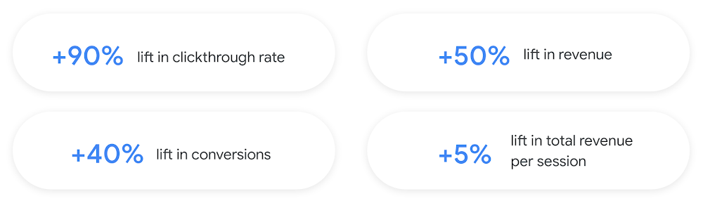
Once models are ready to serve, consider setting up A/B experiments to understand how newly trained models impact your customer experience before serving them to 100% of your traffic. In the Recommendations AI console, see the Monitoring & Analytics page for summary and placement-specific metrics (e.g., recommender-engaged revenue, click-through-rate, conversion rate, and more).
Why use this approach and who is it a good fit for?
Recommendations AI is a great way to engage customers and grow your online presence through personalization. It’s used by teams who lack technical experience with production recommendation systems, as well as customers who have this technical depth but want to allocate their team’s effort towards other priorities and challenges. No matter your team’s technical experience or bandwidth, you can expect several benefits with Recommendations AI:
- Fully managed service: no need to preprocess data, train or hypertune machine learning models, load balance or manually provision you infrastructure – this is all taken care of for you. The recommendation API also provides a user-friendly console to monitor performance over time.
- State-of-the-art AI: take advantage of the same modeling techniques used to serve recommendations across Google Ads, Google Search, and YouTube. These models excel in scenarios with long-tail products and cold-starts users and items
- Deliver at any touchpoint: serve high-quality recommendations to both first-time users and loyal customers anywhere in their journey via web, mobile, email, and more
- Deliver globally: serve recommendations in any language anywhere in the world at low-latency with a fully automated global serving infrastructure
- Your data, your models: Your data and models are yours. They’ll never be used for any other Google product nor shown to any other Google customer
For users looking to leverage state of the art AI to fuel their recommendation systems but need an existing solution to get up and running more quickly, Recommendations AI is the right solution for you.
What are Two Tower encoders and how do they work?
As a reminder, in recommendation system design, our objective is to surface the most relevant set of items for a given user or set of users. The items are usually referred to as the candidate(s) where we might include information about the items such as the title or description of the item, other metadata about the item like language, number of views, or even clicks on the item over time. User(s) are often represented in the form of a query to a recommendation system where we might provide details about the user such as the location of the user, preferred languages, and what they have searched for in the past.
Let’s start with a common example. Imagine that you are creating a movie recommendation system. The input candidates for such a system would be thousands of movies and the query set can consist of millions of viewers. The goal of the retrieval stage is to select a smaller subset of movies(candidates) for each user and then score and rank order them before presenting the final recommended list to the query/user.
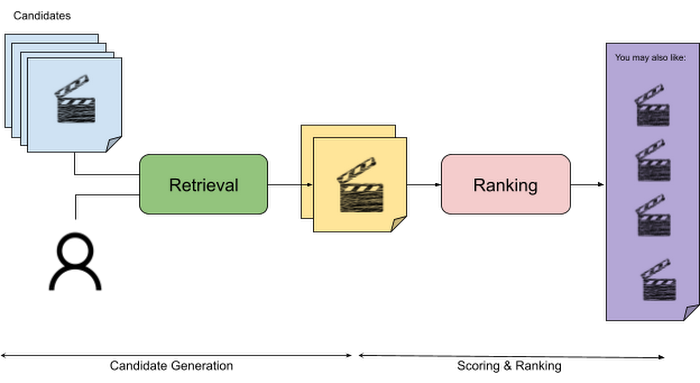
The retrieval stage is able to refine our list of candidates by encoding both the candidate and the query data so they share the same embedding space. A good embedding space will place candidates which are similar to one another closer together and dissimilar items/queries farther apart in the embedding space.
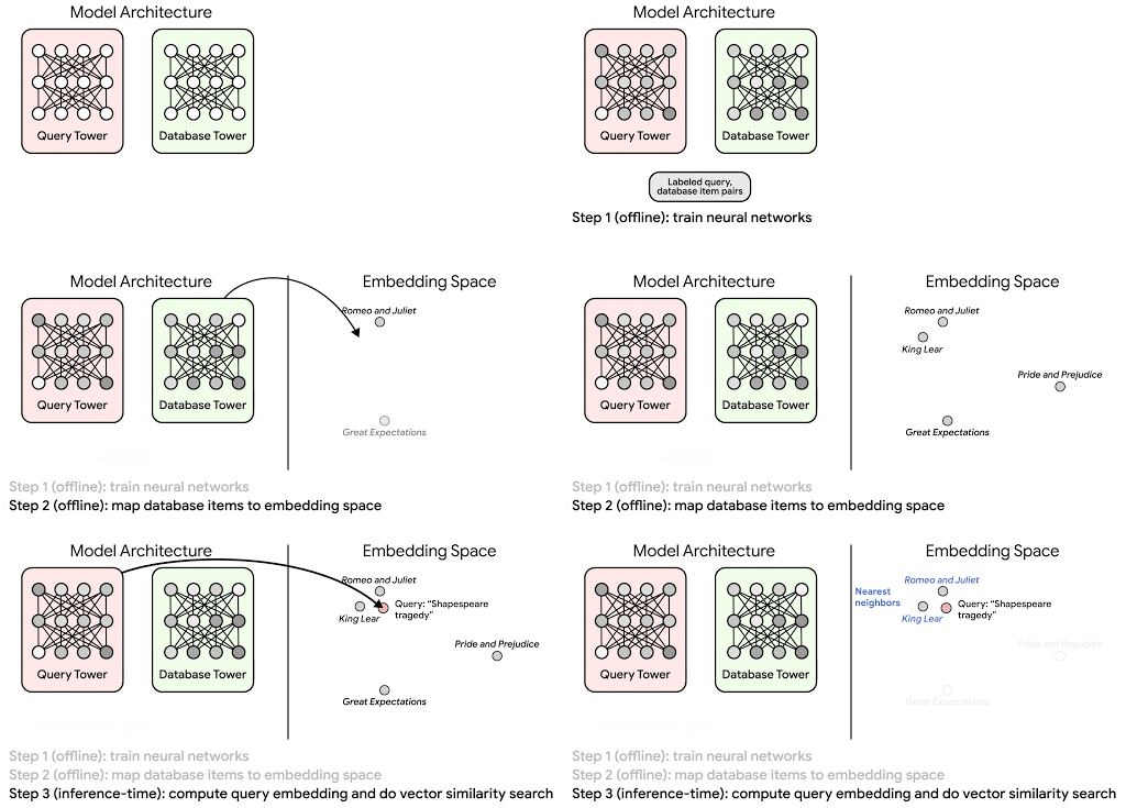
Once we have a database of query and candidate embeddings we can then use an approximate nearest neighbor search method to then generate a list of final “like” candidates, i.e. find a certain number of nearest neighbors for a given query/user and surface final recommendations.
What’s required to get started?
At the most basic level, in order to train a two-tower model you need the following inputs:
- Training Data: Training data is created by combining your query/user data with data about the candidates/items. The data must include matched pairs, cases where both user and item information is available. Data in the training set can include many formats from text, numeric data, or even images.
- Input Schema: The input schema describes the schema of the combined training data along with any specific feature configurations.
Several services within Vertex AI have come available that complement the existing Two-Tower built-in algorithm and can be leveraged in your execution:
- Nearest Neighbor (ANN) Service: Vertex AI Matching Engine and ScANN provide a high-scale and low-latency Approximate Nearest Neighbor (ANN) service so you can more easily identify similar embeddings.
- Hyperparameter Tuning Service: A hyperparameter tuning service such as Vizier can help you identify the optimal hyperparameters such as the number of hidden layers, the size of the hidden layers, and the learning rate in fewer trials.
- Hardware Accelerators: Specialized hardware, such as GPUs or TPUs, can be valuable in your recommendation system to help accelerate experiments and improve the speed of training cycles.
Why use this approach and who is it a good fit for?
The Two-Tower built-in algorithm can be considered the “custom sports car” of recommendation systems and comes with several benefits:
- Greater Control: While Recommendations AI uses the two-tower architecture as one of the available architectures it doesn’t provide granular control or visibility into model training, example generation, and model validation details. In comparison, the Two-Tower built in algorithm provides a more customizable approach as you are training a model directly in a notebook environment.
- More Feature Options: The Two Tower approach can handle additional contextual signals ranging from text to images.
- Cold Start Cases: Leveraging a rich set of features not only enhances performance but also allows the candidate generation to work for new users or new candidates.
While the Two-Tower built in algorithm is an excellent and best-in class solution for deriving recommendations, it does come with additional considerations and potential drawbacks depending upon the use case.
- Technical ML Expertise Required: Two tower encoders are not a “plug and play” solution like the other approaches mentioned above. In order to effectively leverage this approach, appropriate coding and ML expertise is required.
- Speed to Insight: Building out a custom solution via two-tower encoders may require additional time as the solution is not pre-built for the user.
For users looking for greater control, increased flexibility, and have the technical chops to easily work within a managed notebook environment – the two-tower built in algorithm is the right solution for them.
What’s next?
In this article, we explored three common methods for building recommendation systems on Google Cloud Platform. As you can see thus far, there are alot of considerations to take into account before choosing a final approach. In an effort to help you align more quickly we have distilled the decision criteria down to a few simple steps (see below for more details).
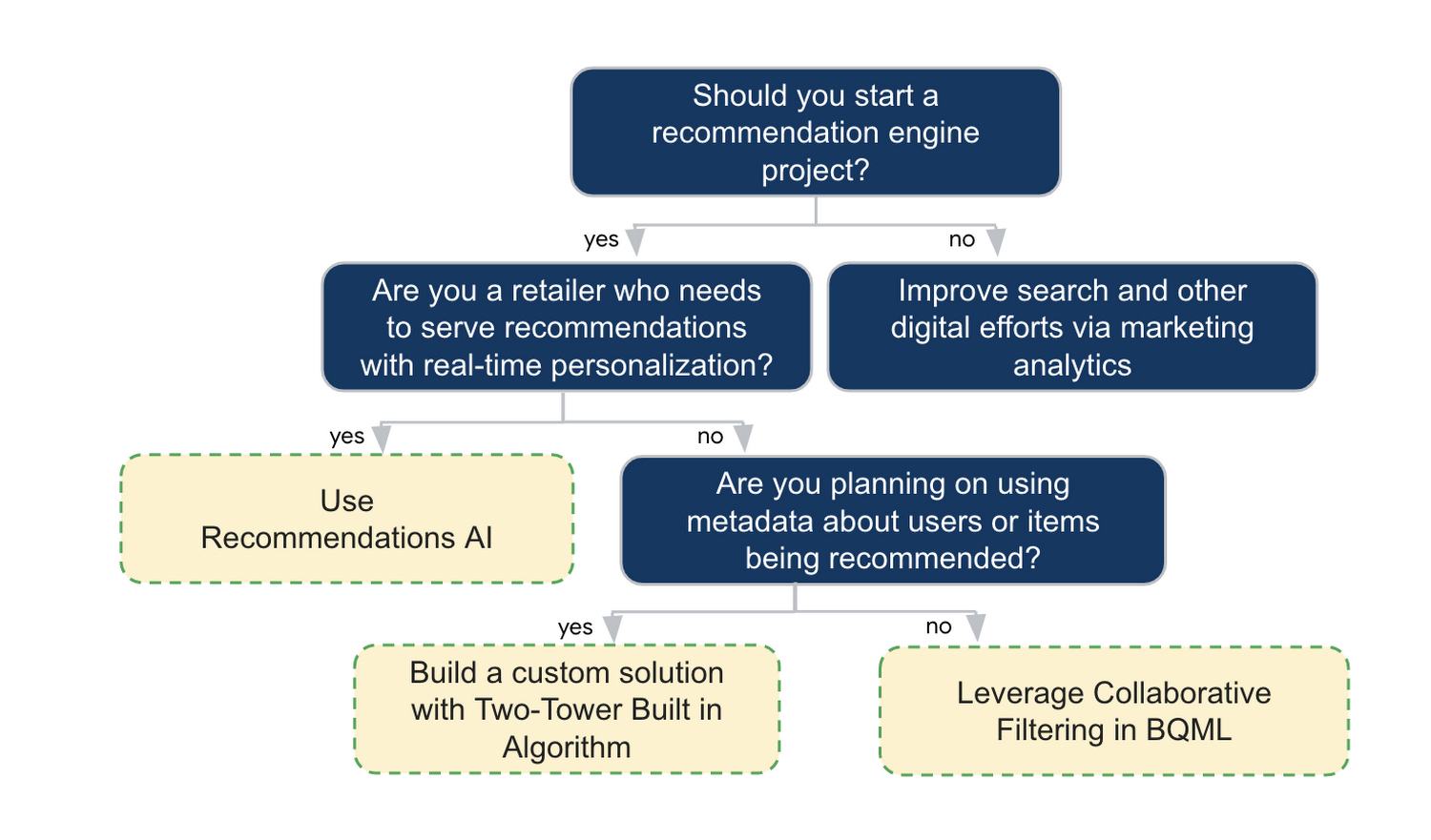
In the next installments of this series, we will dive more deeply into each method, explore how hardware accelerators can play a key role in recommendation system design, and discuss how recommendation systems may be leveraged in key verticals. Stay tuned for future posts in our recommendation systems series. Thank you for reading! Have a question or want to chat? Find authors here – R.E. [Twitter | LinkedIn], Jordan [LinkedIn], and Vaibhav [LinkedIn].
Acknowledgements
Special thanks to Pallav Mehta, Henry Tappen,Abhinav Khushraj, and Nicholas Edelman for helping to review this post.
References
Creating and Using Storage Buckets for Your Data Needs

1389
Of your peers have already read this article.
2:30 Minutes
The most insightful time you'll spend today!
So, you want to store objects on the cloud? But you’re really new to Google Cloud or Cloud Storage and would like someone to walk you through the process step by step?
Today is your lucky day!
I will help you understand the big steps involved in setting up and using Cloud Storage. For a walkthrough of all the steps involved that even includes highlighting of things to select so you don’t spend all your time playing “Where’s Waldo” on the page looking for that one button, click try the tutorial!
Creating buckets, storing objects in them, and adjusting permissions may feel challenging at first, but after you’ve walked through these steps, you’ll be able to create and use the Cloud Storage your project needs.
Resource Hierarchy
Projects contain all of the related parts of your application. Inside projects, you may have buckets, the top level containers in Cloud Storage. Files and folders are stored in buckets. You can grant access to a bucket, folder, or file using Identity and Access Management.
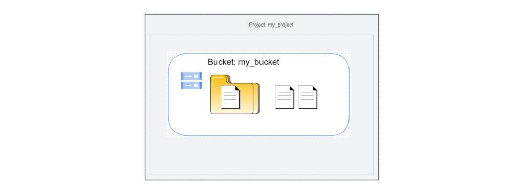
You can do all of that in this interactive tutorial. So let’s get started. I suggest you follow along in the tutorial so you can see the specific keys and screens as I describe them.
Creating a project
Everything in your application will be in a project, even if the only service you are using is storage. Projects need to be associated with a billing account, so if you don’t have one, consider signing up for the Free Trial. You’ll start in the Cloud Console.
Creating a bucket
Once you have a project, you can use storage by navigating to the Cloud Storage page by using either the Navigation menu at the top left of the console or by searching for “Cloud Storage” using the search box at the top of the console.
At the Buckets page of Cloud Storage, you’ll be able to create a bucket. The name of your bucket needs to be globally unique; that is no other bucket in Google Cloud Storage can have the same name. This is because if you or your organization allow your bucket to be accessible on the Internet, it will be at the URL https://storage.googleapis.com/<bucket name>. You can also consider implementing a security feature to prevent data exfiltration, organization restriction headers when you’re finished creating your bucket.. Pick a region close to you for your bucket. In some cases it may make sense to use multi-region or dual-region, but the details are more than I want to get into here. Don’t worry; you can find lots more information on them! Additionally, I won’t go into the details about selecting the appropriate storage class based on access frequency and longevity, but more information can be found here as well our recently introduced Autoclass tiering feature..
Since buckets can be accessed from the Internet, you need to be careful to only make the things you want to be public, public. The default value is to keep your data off of the Internet, so when you create the bucket, there’s an option to “Enforce public access prevention on this bucket” that is already selected. Since we’ll be making items in this bucket public later on, clear the option before confirming the bucket information. Don’t worry; you’ll see how to set that option back later.
Take a look at the Bucket detail page. There are tabs to see the objects in the bucket, the permissions on the bucket, and much more. There are commands to create folders and to upload files and folders. We’ll do some of this in the next section. You can even find out much more from the Learn option in the upper right.
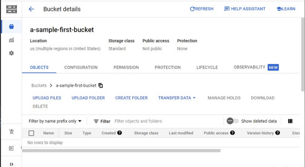
Adding items to the bucket
Find a file you’d like to upload to this bucket, remembering it will be made public to the Internet later. If you don’t have anything available, there’s a picture of a cat (of course, it’s a cat picture, this is the Internet!) in the interactive tutorial.
Go to the bucket details for your bucket. Using the “Upload files” button, you’ll just upload the file to the bucket by selecting the file from your computer. We won’t get into service classes here, but when you’re ready, there are links in the references.
Of course, if you have a lot of files in a bucket, you probably will want some sort of organization. You can do this by creating folders in your bucket with the “Create Folder” option. Once you’ve done that, you can go to the overflow menu (three vertical dots at the end line with the object information) and select Move. Remember, if you need help finding this, the interactive tutorial will point it out.
Making a bucket public
No surprise, the Bucket details hold lots of information about your bucket. You’ll change the bucket’s permissions in the Permission tab. (I hope that’s not a surprise.) You can then give access to individuals, groups, or all users. For this tutorial, follow the steps to grant access to allUsers. There are a variety of different levels of access you can grant to a user. In this case, just grant the ability to view the object using Storage Object Viewer.
Then go into the Objects tab to find the URL for the object you uploaded. Copy that URL and ensure you can indeed access the object from another tab or incognito window.
Now that you’ve done that, go back to the Permission tab for the bucket and select Prevent Public Access to secure the bucket again.
So, in a nutshell, to make all files in a bucket public, in the Permissions tab:
- Uncheck the option “Remove Public Access Prevention”
- Use Grant Access to give allUsers the Storage Object Viewer role in Cloud Storage.
To make all files in a bucket private, in the Permissions tab select Prevent Public Access.
Cleaning up
There is a charge to keep items in Cloud Storage, so you’ll probably want to delete the object you uploaded by selecting it and pressing Delete. You can delete the bucket in a similar way. The tutorial has details, of course.
While there are lots more details about Cloud Storage, you’ve got the big picture now. Go do something creative and useful with it!
So what now?
If you haven’t walked through the interactive tutorial, give it a try!
More Relevant Stories for Your Company

Google’s Anti-Pattern Recognition Tool: Streamlining BigQuery Performance
Why do we need a BigQuery anti-pattern recognition tool? BigQuery is a serverless and cost-effective enterprise data warehouse that works across cloud environments and scales with your data. As with any large scale data-intensive platform, following best practices and avoiding inefficient anti-patterns goes a long way in terms of performance and cost

Demystifying Transactional Locking in Cloud Spanner
Cloud Spanner is a fully managed relational database with unlimited scale, strong consistency, and up to 99.999% availability. It is designed for highly concurrent applications that read and update data, for example, to process payments or for online game play. To ensure the consistency across multiple concurrent transactions, Cloud Spanner

Benefits of BigQuery for SAP Customers
IDC recently examined the benefits of implementing BigQuery for SAP data. The findings reveal massive improvements to the SAP customers' overall business results due to faster access to data insights, lower data warehouse operation cost, and increased productivity among the data warehouse and development teams. Download the report now!

Move over Myths! Here’s What You Need to Know about Cloud Spanner
Intro to Cloud Spanner Cloud Spanner is an enterprise-grade, globally distributed, externally consistent database that offers unlimited scalability and industry-leading 99.999% availability. It requires no maintenance windows and offers a familiar PostgreSQL interface. It combines the benefits of relational databases with the unmatched scalability and availability of non-relational databases. As organizations
