





Optimizing Terabyte-scale PostgreSQL Migrations to Cloud SQL Using Searce

3032
Of your peers have already read this article.
2:30 Minutes
The most insightful time you'll spend today!
Google Cloud allows you to move your PostgreSQL databases to Cloud SQL with Database Migration Service (DMS). DMS gives you the ability to replicate data continuously to the destination database, while the source is live in production, enabling you to migrate with minimum downtime.
However, terabyte-scale migrations can be complex. For instance, if your PostgreSQL database has Large Objects, then you will require some downtime to migrate them manually as that is a limitation of DMS. There are few more such limitations – check out known limitations of DMS. If not handled carefully, these steps can extend the downtime during cutover, lead to performance impact on the source instance, or even delay the project delivery date. All this may mean significant business impact.
Searce is a technology consulting company, specializing in modernizing application and database infrastructure by leveraging cloud, data and AI. We empower our clients to accelerate towards the future of their business. In our journey, we have helped dozens of clients migrate to Cloud SQL, and have found terabyte-scale migrations to be the toughest for the reasons mentioned earlier.
This blog centers around our work in supporting an enterprise client whose objective was to migrate dozens of terabyte scale, mission-critical PostgreSQL databases to Cloud SQL with minimum downtime. Their largest database was 20TB in size and all the databases had tables with large objects and some tables did not have primary keys. Note that DMS had a limitation of not supporting migration of tables without a primary key during the time of this project. In June 2022, DMS released an enhancement to support the migration of tables without a primary key.
In this blog, we share with you our learnings about how we simplified and optimized this migration, so that you can incorporate our best practices into your own migrations. We explore mechanisms to reduce the downtime required for operations not handled by DMS by ~98% with the use of automation scripts. We also explore database flags in PostgreSQL to optimize DMS performance and minimize the overall migration time by ~15%.
Optimize DMS performance with database flags
Once the customer made the decision to migrate PostgreSQL databases to Google Cloud SQL, we considered two key factors that would decide business impact – migration effort and migration time. To minimize effort for the migration of PostgreSQL databases, we leveraged Google Cloud’s DMS (Database Migration Service) as it is very easy to use and it does the heavy lifting by continuously replicating data from the source database to the destination Cloud SQL instance, while the source database is live in production.
How about migration time? For a terabyte-scale database, depending on the database structure, migration time can be considerably longer. Historically, we observed that DMS took around 3 hours to migrate a 1 TB database. In other cases, where the customer database structure was more complex, migration took longer. Thankfully, DMS takes care of this replication while the source database is live in production, so no downtime is required during this time. Nevertheless, our client would have to bear the cost of both the source and destination databases which for large databases, might be substantial. Meanwhile, if the database size increased, then replication could take even longer, increasing the risk of missing the customer’s maintenance window for the downtime incurred during cutover operations. Since the customer’s maintenance window was monthly, we would have to wait for 30 more days for the next maintenance window, requiring the customer to bear the cost of both the databases for another 30 days. Furthermore, from a risk management standpoint, the longer the migration timeframe, the greater the risk that something could go wrong. Hence, we started exploring options to reduce the migration time. Even the slightest reduction in migration time could significantly reduce the cost and risk.
We explored options around tuning PostgreSQL’s database flags on the source database. While DMS has its own set of prerequisite flags for the source instance and database, we also found that flags like shared_buffers, wal_buffers and maintenance_work_mem helped accelerate the replication process through DMS. These flags needed to be set to a specific value to get the maximum benefit out of each of them. Once set, their cumulative impact was a reduction in time for DMS to replicate a 1 TB database by 4 hours, that is, reduction of 3.5 days for a 20 TB database. Let’s dive into each of them.
Shared Buffers
PostgreSQL uses two buffers – its own internal buffer and the kernel buffered IO. In other words, that data is stored in memory twice. The internal buffer is called shared_buffers, and it determines the amount of memory used by the database for the operating system cache. By default this value is set conservatively low. However, increasing this value on the source database to fit our use case helped increase the performance of read heavy operations, which is exactly what DMS does once a job has been initialized.
After multiple iterations, we found that if the value was set to 55% of the database instance RAM, it boosted the replication performance (a read heavy operation) by a considerable amount and in turn reduced the time required to replicate the data.
WAL Buffers
PostgreSQL relies on Write-Ahead Logging (WAL) to ensure data integrity. WAL records are written to buffers and then flushed to disk. The flag wal_buffers, determines the amount of shared memory used for WAL data that has not yet been written to disk – records that are yet to be flushed. We found that increasing the value for wal_buffers from the default value of 16MB to about 3% of the database instance’s RAM significantly improved the write performance by writing fewer but larger files to the disk at each transaction commit.
Maintenance Work Mem
PostgreSQL maintenance operations, such as VACUUM, CREATE INDEX, and ALTER TABLE ADD FOREIGN KEY, consume their own specific memory. This memory is referred to as maintenance_work_mem. Unlike other operations, PostgreSQL maintenance operations can only be performed sequentially by the database. Setting a value significantly higher than the default value of 64 MB meant that no maintenance operation would block the DMS job. We found that maintenance_work_mem worked best at the value of 1 GB.
Resize source instance to avoid performance impact
Each of these three flags tune how PostgreSQL utilizes memory resources. Hence, it was imperative that before setting these flags, we needed to upsize the source database instance to accommodate them. Without upsizing the database instances, we could have caused application performance degradation, as more than half of the total database memory would be allocated to the processes managed by these flags.
We calculated the memory required by the flags mentioned above, and found that each flag needed to be set to a specific percentage of the source instance’s memory, irrespective of the existing values that might be set for the flags:
- shared_buffers: 55% of source instance’s memory
- wal_buffers: 3% of source instance’s memory
- maintenance_work_mem: 1 GB
We added the individual memory requirements by the flags, and found that 58% of the RAM at least will be taken up by these memory flags. For example, if a source instance used 100GB of memory, 58GB would be taken up by shared_buffers and wal_buffers, and an additional 1GB by maintenance_work_mem. As the original value of these flags was very low (~200MB), we upsized the RAM of the source database instance by 60% in order to ensure that the migration did not impact source performance on the application live in production.
Avoid connection error with WAL sender timeout flag
While using Google Cloud’s DMS, if the connection is terminated between DMS and the Cloud SQL instance during the ‘Full Dump in Progress’ phase of the DMS job, the DMS job fails and needs to be reinitiated. Encountering timeouts, especially while migrating a terabyte-scale database, would mean multiple days’ worth of migration being lost and a delay in the cutover plan. For example, if the connection of the DMS job for a 20TB database migration is lost after 10 days, the DMS job will have to be restarted from the beginning, leading to 10 days’ worth of migration effort being lost.
Adjusting the WAL sender timeout flag (wal_sender_timeout) helped us avoid terminating replication connections that were inactive for a long time during the full dump phase. The default value for this flag is 60 seconds. To avoid these connections from terminating, and to avoid such high impact failures, we set the value of this flag to 0 for the duration of database migration. This would avoid connections getting terminated and allowed for smoother replication through the DMS jobs.
Generally, for all the database flags we talked about here, we advised our customer to restore the default flag values once the migration completed.
Reduce downtime required for DMS limitations by automation
While DMS does the majority of database migration through continuous replication when the source database instance is live in production, DMS has certain migration limitations that cannot be addressed when the database is live. For PostgreSQL, the known limitations of DMS include:
- Any new tables created on the source PostgreSQL database after the DMS job has been initialized are not replicated to the destination PostgreSQL database.
- Tables without primary keys on the source PostgreSQL database are not migrated. For those tables, DMS migrated only the schema. This is no longer a limitation after the June 2022 product update.
- The large object (LOB) data type is not supported by DMS.
- Only the schema for Materialized Views is migrated; the data is not migrated.
- All data migrated is created under the ownership of cloudsqlexternalsync.
We had to address these aspects of the database migration manually. Since our client’s database had data with the large object data type, tables without primary keys, and frequently changing table structures that cannot be migrated by DMS, we had to manually export and import that data after DMS did most of the rest of the data migration. This part of database migration required downtime to avoid data loss. For a terabyte-scale database, this data can be in the hundreds of GBs, which means higher migration time and hence higher downtime. Furthermore, when you have dozens of databases to migrate, it can be stressful and error-prone for a human to perform these operations while on the clock during the cutover window!
This is where automation helped save the day! Automating the migration operations during the downtime period not only reduced the manual effort and error risk, but also provided a scalable solution that could be leveraged for the migration of 100s of PostgreSQL database instances to Cloud SQL. Furthermore, by leveraging multiprocessing and multithreading, we were able to reduce the total migration downtime for 100s of GBs of data by 98%, thereby reducing the business impact for our client.
How do we get there?
We laid out all the steps that need to be executed during the downtime – that is, after the DMS job has completed its replication from source to destination and before cutting over the application to the migrated database. You can see a chart mapping out the sequence of operations that are performed during the downtime period in Fig 1.
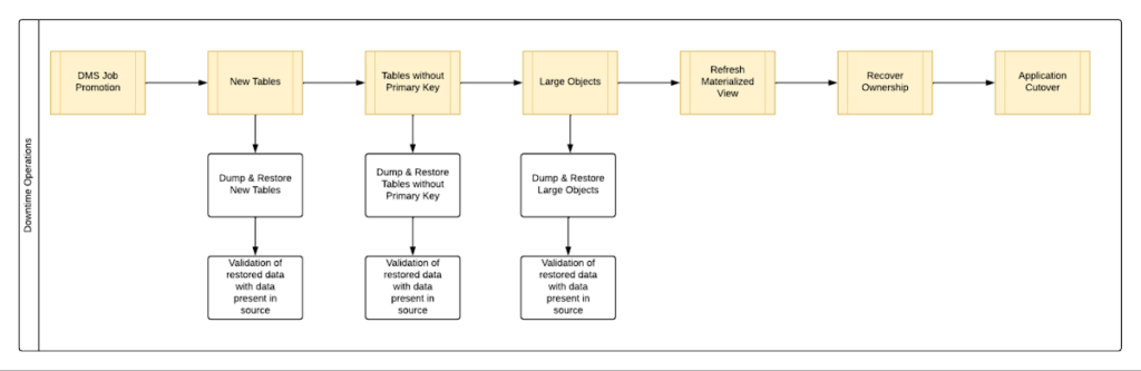
By automating all the downtime operations in this sequential approach, we observed that it took 13 hours for the entire downtime flow to execute for a 1 TB database. This included the migration of 250 MB in new tables, 60 GB in tables without primary keys and 150 GB in large objects.
One key observation we made was that, out of all the steps, only three steps took most of the time: migrating new tables, migrating tables without primary keys, and migrating large objects. These took the longest time because they all required dump and restore operations for their respective tables. However, these three steps did not have a hard dependency on each other as they individually targeted different tables. So we tried to run them in parallel as you can see in Fig 2. But the steps following them – ‘Refresh Materialized View’ and ‘Recover Ownership’ – had to be performed sequentially as they targeted the entire database.
However, running these three steps in parallel required upsizing the Cloud SQL instances, as we wanted to have sufficient resources available for each step. This led us to increase the Cloud SQL instances’ vCPU by 50% and memory by 40%, since the export and import operations depended heavily on vCPU consumption as opposed to memory consumption.
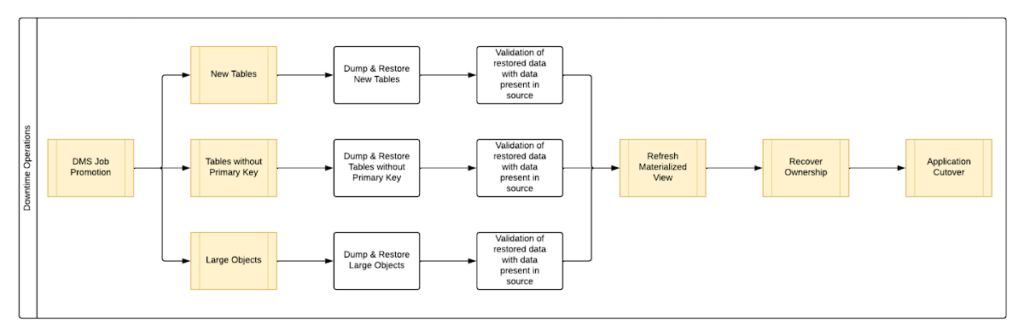
Migrating the new tables (created after the DMS job was initiated) and tables without primary keys was straightforward as we were able to leverage the native utilities offered by PostgreSQL – pg_dump and pg_restore. Both utilities process tables in parallel by using multiple threads– the higher the table count, the higher the number of threads that could be executed in parallel, allowing faster migration. With this revised approach, for the same 1 TB database, it still took 12.5 hours for the entire downtime flow to execute.
This improvement reduced the cutover downtime, but we still found that we needed a 12.5 hour window to complete all the steps. We then discovered that 99% of the time of downtime was taken up by just one step: exporting and importing 150 GB of large objects. It turned out that multiple threads could not be used to accelerate the dump and restore large objects in PostgreSQL. Hence, migrating the large objects single handedly extended the downtime for migration by hours. Fortunately, we were able to come up with a workaround for that.
Optimize migration of Large Object from PostgreSQL database
PostgreSQL contains a large objects facility that provides stream-style access to data stored in a special large-object structure. When large objects are stored, they are broken down into multiple chunks and stored in different rows of the database, but are connected under a single Object Identifier (OID). This OID can thus be used to access any stored Large Object. Although users can add large objects to any table in the database, under the hood, PostgreSQL physically stores all large objects within a database in a single table called pg_largeobjects.
While leveraging pg_dump and pg_restore for export and import of large objects, this single table – pg_largeobject, becomes a bottleneck as the PostgreSQL utilities cannot execute multiple threads for parallel processing, since it’s just one table. Typically, the order of operations for these utilities looks something like this:
- pg_dump reads the data to be exported from the source database
- pg_dump writes that data into the memory of the client where pg_dump is being executed
- pg_dump writes from memory to the disk of the the client (a second write operation)
- pg_restore reads the data from the client’s disk
- pg_restore writes the data to the destination database
Normally, these utilities would need to be executed sequentially to avoid data loss or data corruption due to conflicting processes. This leads to further increase in migration time for large objects.
Our workaround for this single-threaded process involved two elements. First, with our solution, we eliminated the second write operation – write from memory to disk (point #3). Instead, once the data was read and written into memory, our program would begin the import process and write data to the destination database. Second, since pg_dump and pg_restore could not use multiple threads to process the large objects in just the pg_largeobjects table, we took it upon ourselves to develop a solution that could use multiple threads. The thread count was based on the number of OIDs in the table – pg_largeobjects, and break that single table into smaller chunks for parallel execution.
This approach brought down Large Object migration operation from hours to minutes, therefore bringing down the downtime needed for all operations to be completed that DMS cannot handle, for the same 1 TB database, from 13 hours to just 18 minutes. A reduction of ~98% in the required downtime.
Conclusion
After multiple optimizations and dry runs, we were able to develop a procedure for our client to migrate dozens of terabyte-scale PostgreSQL databases to Google Cloud SQL with a minimal business impact. We developed practices to optimize DMS-based migration by 15% using database flags and reduce downtime by 98% with the help of automation and innovation. These practices can be leveraged for any terabyte-scale migration of PostgreSQL databases to Google Cloud SQL to accelerate migration, minimize downtime and avoid performance impact on mission critical applications.
Neo4J & Google Cloud: Graph Data in Cloud to Address Challenges in FinServ Industry

6915
Of your peers have already read this article.
3:00 Minutes
The most insightful time you'll spend today!
Over the last decade, financial service organizations have been adopting a cloud-first mindset. According to InformationWeek, lower costs and enhanced scalability were the biggest drivers for cloud adoption in financial services, and cloud-native applications allow access to the latest technology and talent, enabling adopters to rebuild transaction processing systems capable of supporting very high volumes and low latency.
Both Neo4j and Google Cloud have been using relationship-based data representations since the beginning, and we’re dedicated to using this technology to help financial services customers drive business transformation. We are excited about the prospects of financial services (FinServ) cloud systems and believe that graph data in the cloud can help solve significant challenges in the industry.
Data Challenge #1: Risk Management and Compliance
First among the top concerns for any CIO moving to the cloud is risk management and compliance. Disconnected, uncontextualized, or stale data create opportunities for fraud and financial crimes to occur. The fact is when it comes to FinServ, the question is not “if” but rather how often an attack will occur. Unfortunately, incidents have been trending upward over the last decade, and COVID has only exacerbated this reality. Financial crimes affect the bottom line both in the remediation of these crimes and in intangibles like brand value.
Add to this the complexity of international banking, which makes “compliance” a moving target. Penalties due to noncompliance are a constant concern to any FinServ organization.
The tabular representation of information with a fixed number of columns that never change prevents a description of an ever changing world with changing characteristics. Relational databases are great if the world you describe does not move fast but have limitations when data structures are highly interlinked and not homogeneous.
Neo4j Aura on Google Cloud provides a foundation for creating dynamic, futureproof, scalable applications that adhere to the security standards and protocols today’s financial services organizations require to meet the challenges of finding and preventing bad actors. This also includes enterprise scalability; reaching over 1 Billion nodes and relationships to streamline queries and provide solutions that meet regulatory and privacy compliance across geographies. Neo4j has helped some organizations save billions of USD in fraud in the first year of deployment alone.
What makes graph technology the best choice for fraud detection use cases is that the relationships between the data-points are as important as the data-points themselves. Let’s take as an example, one John Smith approaches a multi-national banking institution to manage the primary account for his new holding corporation.
While no one has any record of John R Smith Holdings LLC, the bank’s application built on graph technology understands that there are several well-known entities owned by John Smith Holdings. The application also identifies several well-known board members who bank with this institution. Due to this relationship-driven approach, the bank now understands John R Smith is not “John Smith,” who previously attempted to open an account for his holding corporation, which had no information associated with it prior to two months ago.
Data Challenge #2 Manual Processes and Inefficiencies
The ubiquity of the cloud offers an opportunity to deploy automation at unprecedented levels to tackle the errors and inefficiencies that manual processing allows to creep into processes. When data comes from disparate, perhaps legacy systems – which may have become siloed and “untouchable” over the years – further complexity arises. As an example, if someone in sales types “John Smith” into a CRM system not knowing that John R Smith is the spelling in the customer data master, it may result in two separate and potentially conflicting records. Being able to join those records together in a mastered view helps to solve this problem. In addition, low data quality equates to an increase in risk, costs, and implementation times for new systems.
Neo4j Aura on Google Cloud provides automation and artificial intelligence (AI) that reduces manual processes and the errors that accompany them. In this graph architecture each node, which can represent a person, will have labels, relationships, and properties associated with it. This allows for the use of AI which can easily understand that John Smith in the CRM is the same John R Smith in the customer master. The information contained in Neo4j can be connected bi-directionally to ensure consistency across applications and data sources.
One of the benefits of this approach is that linking information allows organizations to keep the full value of the data, rather than forcing the data into predetermined tabular representations, with the risk of losing valuable information and insights.
Data Challenge #3: Customer Engagement and Insight
Another significant concern is the high expectations today’s customers have for every interaction. End users are accustomed to predictable experiences on their digital devices, and FinServ apps are no exception. Added to this, the “Covid economy” has driven digital adoption significantly across demographics; even among customers who might traditionally have used in-person services. This also equates to increased expectations for personalized, predictable experiences with every digital interaction. We know that latency has always been a key consideration for financial trading, but a recent ComputerWeekly study showed that every financial organization should ensure their visible latency is at 10 milliseconds or less. Customers no longer accept their broadband is at fault.
Finally, blind spots in the customer journey often result in dissatisfaction, which ultimately leads to increased churn. Without gaining actionable insights from your customers, there is no room to innovate and iterate on what they are looking for in your products and services. And this translates to losing market share and competitive advantage.
The NoSQL architecture, specifically the dynamic schema and structure of Neo4j Aura gives you the ability to take charge of your data and make changes according to your development cycles or newer data models. This equates to faster builds, more comprehensive releases and a wider, richer data-set that can be contextualized and understood instantly. Graph technology is the logical choice for building a Customer 360 application. Under this approach organizations not only get valuable insight into the individual client’s behavior and patterns, but also those of their family, friends and colleagues. This allows for stronger personalization, targeted campaigns and successful execution, resulting in increased customer satisfaction and retention levels.
Graph Technology on Google Cloud

Neo4j is a recognized leader in graph database technology and the only fully integrated graph solution on Google Cloud, helping to fill a common need for Google Cloud customers. Both Neo4j and Google Cloud are invested in continuing to grow our partnership and mutual product direction.
You can find and deploy the Neo4j graph database straight from the Google Cloud marketplace, whether you want to download the software for an on-premises deployment, use the virtual machine image, or use the hosted solution, Aura on Google Cloud, the graph database-as-a-service. In any deployment, you get the same enterprise-grade scalability, reliability, and connectivity along with successful, repeatable use cases you can rely on to resolve your particular challenges and integrated billing.
For a real-world example of how graph technology can optimize financial services, you can read our Case Study with fintech Current. Current, a leading U.S. financial technology platform with over three million members, used Neo4j Aura on Google Cloud to create a personalization engine based on client relationships.
To learn more about Neo4j Aura on Google Cloud for FinServ organizations, register for our webinar on Thursday, December 16 with Jim Webber, Chief Scientist, CTO Field Ops at Neo4j and Antoine Larmanjat, Technical Director, Office of the CTO, Google Cloud.
Maximizing Storage Efficiency: A Guide to Reducing Point-in-Time Recovery Impact

1468
Of your peers have already read this article.
1:30 Minutes
The most insightful time you'll spend today!
Point-In-Time Recovery (PITR) is a critical capability for enterprise applications. It allows database administrators to recover from accidental data deletion by restoring their production databases to a time before the incident.
Cloud SQL for PostgreSQL launched support for PITR in July 2020, allowing you to recover from disasters like data corruption or accidental deletion by restoring your Cloud SQL instance to a previous time. We’re excited to announce an additional enhancement to PITR for Cloud SQL for PostgreSQL that makes enabling PITR an even easier decision: for instances with Point-in-Time Recovery newly-enabled, the write-ahead logs being stored for PITR operations (which are the transaction logs that are used to go back in time) will no longer consume disk storage space. Instead, when you enable PITR for new instances, Cloud SQL will store transaction logs collected during the retention window in Google Cloud Storage, and retrieve them when you perform a restore. Because transaction logs can grow rapidly when your database experiences a burst of activity, this move will help reduce the impact these bursts have on your provisioned disk storage. These logs will be stored for up to seven days in the same Google Cloud region as your instance at no additional cost to you.
PITR is enabled by default when you create a new Cloud SQL for PostgreSQL instance from the Google Cloud console, and transaction logs will no longer be stored on the instance for instances that have PITR newly enabled. If you have already enabled PITR on your PostgreSQL instances, this enhancement will be rolled out to your instances at a later point. If you want to take advantage of this change sooner, you can first disable and then re-enable PITR on your instance (which will reset your ability to perform a point-in-time restore to the time at which PITR was re-enabled). On instances with this feature enabled, you’ll notice that consumed storage on your instance will reduce relative to the volume of write-ahead logs (WAL) generated by your instance. The actual amount of storage your logs consume will vary by instance and by database activity – during busy times for your database, log size may shrink or grow. However, these logs will now only be stored on your instance long enough to successfully replicate to any replicas of the instance and to ensure that they are safely written to Cloud Storage; afterwards, they will be removed from your instance.
We’re excited to continue to enhance Cloud SQL for PostgreSQL to ensure that disaster recovery is easy to enable, cost effective, and seamless to use. Learn more about this change in our documentation.
Spot Slow MySQL Queries Fast with Stackdriver Monitoring

4042
Of your peers have already read this article.
4:30 Minutes
The most insightful time you'll spend today!
When you’re serving customers online, speed is essential for a good experience. As the amount of data in a database grows, queries that used to be fast can slow down.
For example, if a query has to scan every row because a table is missing an index, response times that were acceptable with a thousand rows can turn into multiple seconds of waiting once you have a million rows.
If this query is executed every time a user loads your web page, their browsing experience will slow to a crawl, causing user frustration. Slow queries can also impact automated jobs, causing them to time out before completion.
If there are too many of these slow queries executing at once, the database can even run out of connections, causing all new queries, slow or fast, to fail.
The popular open-source databases MySQL and Google Cloud Platform‘s fully managed version, Cloud SQL for MySQL, include a feature to log slow queries, letting you find the cause, then optimize for better performance.
However, developers and database administrators typically only access this slow query log reactively, after users have seen the effects and escalated the performance degradation.
With Stackdriver Logging and Monitoring, you can stay ahead of the curve for database performance with automatic alerts when query latency goes over the threshold, and a monitoring dashboard that lets you quickly pinpoint the specific queries causing the slowdown.
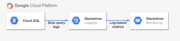
To get started, import MySQL’s slow query log into Stackdriver Logging.
Once the logs are in Stackdriver, it’s straightforward to set up logs-based metrics that can both count the number of slow queries over time, which is useful for setting up appropriate alerts, and also provide breakdowns by slow SQL statement, allowing speedy troubleshooting.
What’s more, this approach works equally well for managed databases in Cloud SQL for MySQL and for self-managed MySQL databases hosted on Compute Engine.
For a step-by-step tutorial to set up slow query monitoring, check out Monitoring slow queries in MySQL with Stackdriver. For more ideas about what else you can accomplish with Stackdriver Logging, check out Design patterns for exporting Stackdriver Logging.
Simplifying Unstructured Data Analytics with BigQuery ML and Vertex AI: A Comprehensive Guide

1556
Of your peers have already read this article.
6:30 Minutes
The most insightful time you'll spend today!
Unstructured data such as images, speech and textual data can be notoriously difficult to manage, and even harder to analyze. The analysis of unstructured data includes use cases such as extracting text from images using OCR, sentiment analysis on customer reviews and simplifying translation for analytics. All of this data needs to be stored, managed and made available for machine learning.
The new BigQuery ML inference engine empowers practitioners to run inferences on unstructured data using pre-trained AI models. The results of these inferences can be analyzed to extract insights and improve decision making. This can all be done in BigQuery, using just a few lines of SQL.
In this blog, we’ll explore how the new BigQuery ML inference engine can be used to run inferences against unstructured data in BigQuery. We’ll demonstrate how to detect and translate text from movie poster images, and run sentiment analysis against movie reviews.
BigQuery ML’s new inference engine
Google Cloud is home to a suite of pre-trained AI models and APIs. The BigQuery ML inference engine can call these APIs and manage the responses on your behalf. All you have to do is define the model you want to use and run inferences against your data. All of this is done in BigQuery using SQL. The inference results are returned in JSON format and stored in BigQuery for analysis.
Why run your inferences in BigQuery?
Traditionally, working with AI models to run inferences required expertise in programming languages like Python. The ability to run inferences in BigQuery using just SQL can make generating insights from your data using AI simple and accessible. BigQuery is also serverless, so you can focus on analyzing your data without worrying about scalability and infrastructure.
The inference results are stored in BigQuery, which allows you to analyze your unstructured data immediately, without the need to move or copy your data. A key advantage here is that this analysis can also be joined with structured data stored in BigQuery, giving you the opportunity to deepen your insights. This can simplify data management and minimize the amount of data movement and duplication required.
Which models are supported?
For now, the BigQuery ML inference engine can be used with these pre-trained Vertex AI models:
- Vision AI API: This model can be used to extract features from images managed by BigQuery Object Tables and stored on Cloud Storage. For example, Vision AI can detect and classify objects, or read handwritten text.
- Translation AI API: This model can be used to translate text in BigQuery tables into over one hundred languages.
- Natural Language Processing API: This model can be used to derive meaning from textual data stored in BigQuery tables. For example, features like sentiment analysis can be used to determine whether the emotional tone of text is positive or negative.
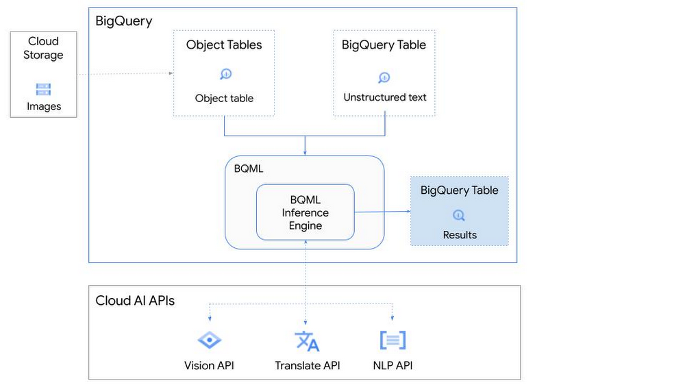
So, how does this work in practice? Let’s look at an example using images of movie posters

- We will define our pre-trained models for Vision AI, Translation AI and NLP AI in BigQuery ML.
- We’ll then use Vision AI to detect the text from some classic movie posters images.
- Next, we’ll use Translation AI to detect any foreign posters and translate them to a language of our choosing – English in this case.
- Finally, we’ll combine our unstructured data with structured data in BigQuery.
We’ll use the extracted movie titles from our movie posters to look up the viewer reviews from the BigQuery IMDB public dataset. We can then run sentiment analysis against these reviews using NLP AI.
Note: The BigQuery ML inference engine is currently in Preview. You will need to complete this enrollment form to have your project allowlisted for use with the BQML Inference Engine.
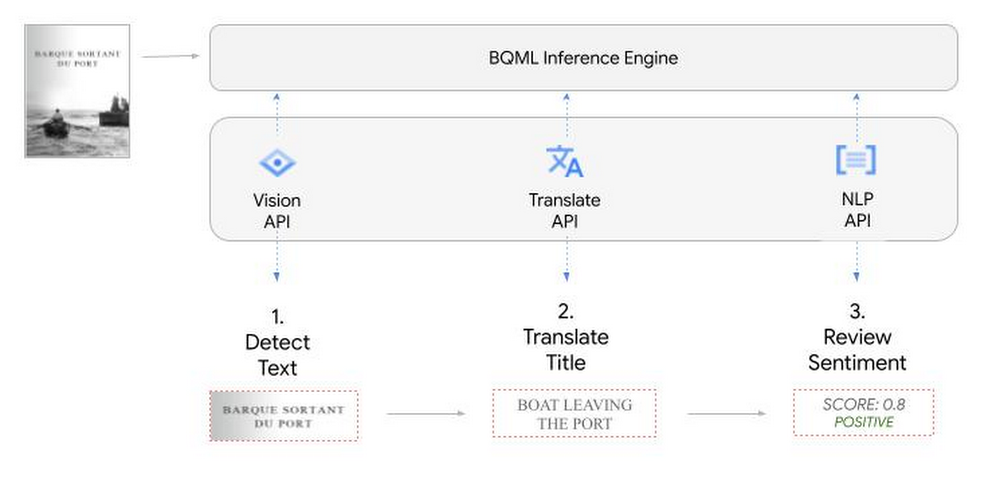
We’ll give examples of the BigQuery SQL needed to define your models and run your inferences. You’ll want to check out our notebook for a detailed guide on how to get this up and running in your Google Cloud project.
1. Define your AI Models in BigQuery
You will need to enable the APIs listed below, and also create a Cloud resource connection to enable BigQuery to interact with these services.
| API | Model Name |
| Vision AI API | Cloud_ai_vision_v1 |
| Translation AI API | Cloud_ai_translate_v3 |
| NLP AI API | Cloud_ai_natural_language_v1 |
You can then run the CREATE MODEL query for each AI service to create your pretrained models, replacing the model_name as required.
CREATE OR REPLACE MODEL
`{PROJECT_ID}.{DATASET_ID}.{VISION_MODEL_NAME}`
REMOTE WITH
CONNECTION `{PROJECT_ID}.{REGION}.{CONN_NAME}`
OPTIONS ( remote_service_type = '<model_name>' );
2. Use the Vision AI API to detect text in images stored in Cloud Storage
You will need to create an object table for your images in Cloud Storage. This read-only object table provides metadata for images stored in Cloud Storage:
CREATE OR REPLACE EXTERNAL TABLE
`{PROJECT_ID}.{DATASET_ID}.{OBJECT_TABLE_NAME}`
WITH
CONNECTION `{REGION}.{CONN_NAME}`
OPTIONS (object_metadata = 'SIMPLE', uris = ['{BUCKET_LOCATION}/*']);
To detect the text from our posters, you can then use ML.ANNOTATE_IMAGE and specify the text_detection feature.
SELECT
       ml_annotate_image_result.full_text_annotation.text AS text_content,
       *
FROM
       ML.ANNOTATE_IMAGE(
         MODEL `{PROJECT_ID}.{DATASET_ID}.{VISION_MODEL_NAME}`,
         TABLE `{DATASET_ID}.{OBJECT_TABLE_NAME}`,
         STRUCT(['TEXT_DETECTION'] AS vision_features));
A JSON response will be returned to BigQuery that includes the text content and language code of the text. You can parse the JSON to a scalar result using the dot annotation highlighted above.

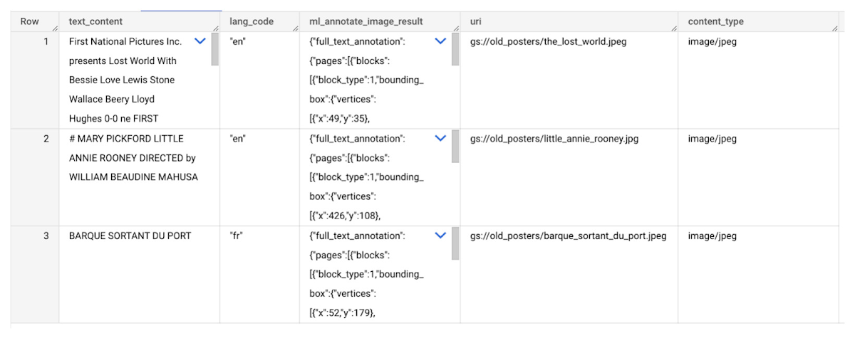
3. Use the Translation AI API to translate foreign movie titles
ML.TRANSLATE can now be used to translate the foreign titles we’ve extracted from our images into English. You just need to specify the target language and the table of the movie posters for translation:
SELECT
text_content,
STRING(ml_translate_result.translations[0].detected_language_code)
as original_language,
STRING(ml_translate_result.translations[0].translated_text)
as translated_title
FROM
  ML.TRANSLATE(
MODEL `{PROJECT_ID}.{DATASET_ID}.{TRANSLATE_MODEL_NAME}`,
TABLE `{DATASET_ID}.image_results`,
STRUCT('TRANSLATE_TEXT' as translate_mode, "en" as target_language_code));
Note: The table column with the text you want to translate must be named text_content:
The table of results will include json that can be parsed to extract both the original language and the translated text. In this case, the model has detected that title text is in French and has translated it to English:

4. Finally, use natural language processing (NLP) to run sentiment analysis against movie reviews
You can easily join inference results from your unstructured data with other BigQuery datasets to bolster your analysis. For example, we can now join the movie titles we extracted from our posters with thousands of movie reviews stored in BigQuery’s IMDB public dataset `bigquery-public-data.imdb.reviews`.
You can use ML.UNDERSTAND_TEXT with the analyze_sentiment feature to run sentiment analysis against some of these reviews to determine whether they are positive or negative:
SELECT
   primary_title, start_year, text_content AS review,
   FLOAT64(ml_understand_text_result.document_sentiment.score) AS score,
   FLOAT64(ml_understand_text_result.document_sentiment.magnitude) AS magnitude,
FROM
   ML.UNDERSTAND_TEXT(
     MODEL `{PROJECT_ID}.{DATASET_ID}.{NLP_MODEL_NAME}`,
           (
           SELECT
             primary_title, start_year, review AS text_content
           FROM
             `bigquery-public-data.imdb.title_basics` titles
           JOIN
             `bigquery-public-data.imdb.reviews` reviews
           ON
             reviews.movie_id = titles.tconst
           WHERE
             UPPER(titles.primary_title) = 'THE LOST WORLD' AND
             start_year = 1925
           ),
      STRUCT("analyze_sentiment" AS nlu_option)) ;
Note: The table column with the text you want to analyze must be named text_content:
The JSON response will include a score and magnitude. The score indicates the overall emotion of the text while the magnitude indicates how much emotional content is present:
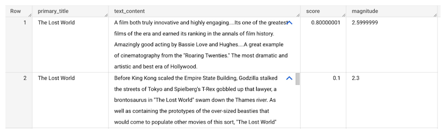
So, how did the Lost World compare with other movies that year?
To wrap up, we’ll compare the average review score of the 1925 Lost World movie to other movies released that year to see which was more popular. This can be done using familiar SQL analysis:
SELECT
 primary_title, start_year,
 AVG(FLOAT64(ml_understand_text_result.document_sentiment.score))AS av_score,
 AVG(FLOAT64(ml_understand_text_result.document_sentiment.magnitude)) AS av_magnitude
FROM
 ML.UNDERSTAND_TEXT(
   MODEL `{PROJECT_ID}.{DATASET_ID}.{NLP_MODEL_NAME}`,
         (
         SELECT
           primary_title, start_year, movie_id, review AS text_content
         FROM
           `bigquery-public-data.imdb.title_basics` titles
         JOIN
           `bigquery-public-data.imdb.reviews` reviews
         ON
           reviews.movie_id = titles.tconst
         WHERE
           start_year = 1925
         ),
   STRUCT("analyze_sentiment" AS nlu_option))
GROUP BY
   primary_title, start_year
ORDER BY
   av_score DESC;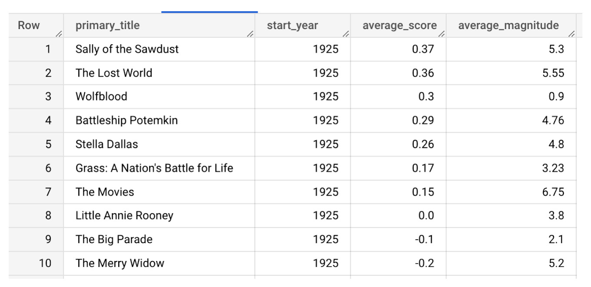
It looks like The Lost World narrowly missed out on the top spot to Sally of the Sawdust!
Want to learn more?
Check out our notebook for a step by step guide on using the BQML inference engine for unstructured data in Google Cloud. You can also check out our Cloud AI service table-valued functions overview page for more details. Curious about pricing? The BQML Pricing page gives a breakdown of how costs are applied across these services.
How to Decide Whether to Run a Database on Kubernetes
5626
Of your peers have already read this article.
3:30 Minutes
The most insightful time you'll spend today!
Today, more and more applications are being deployed in containers on Kubernetes—so much so that we’ve heard Kubernetes called the Linux of the cloud.
Despite all that growth on the application layer, the data layer hasn’t gotten as much traction with containerization. That’s not surprising, since containerized workloads inherently have to be resilient to restarts, scale-out, virtualization, and other constraints. So handling things like state (the database), availability to other layers of the application, and redundancy for a database can have very specific requirements. That makes it challenging to run a database in a distributed environment.
However, the data layer is getting more attention, since many developers want to treat data infrastructure the same as application stacks.
Operators want to use the same tools for databases and applications, and get the same benefits as the application layer in the data layer: rapid spin-up and repeatability across environments. In this blog, we’ll explore when and what types of databases can be effectively run on Kubernetes.
Before we dive into the considerations for running a database on Kubernetes, let’s briefly review our options for running databases on Google Cloud Platform (GCP) and what they’re best used for.
- Fully managed databases. This includes Cloud Spanner, Cloud Bigtable and Cloud SQL, among others. This is the low-ops choice, since Google Cloud handles many of the maintenance tasks, like backups, patching and scaling. As a developer or operator, you don’t need to mess with them. You just create a database, build your app, and let Google Cloud scale it for you. This also means you might not have access to the exact version of a database, extension, or the exact flavor of database that you want.
- Do-it-yourself on a VM. This might best be described as the full-ops option, where you take full responsibility for building your database, scaling it, managing reliability, setting up backups, and more. All of that can be a lot of work, but you have all the features and database flavors at your disposal.
- Run it on Kubernetes. Running a database on Kubernetes is closer to the full-ops option, but you do get some benefits in terms of the automation Kubernetes provides to keep the database application running. That said, it is important to remember that pods (the database application containers) are transient, so the likelihood of database application restarts or failovers is higher. Also, some of the more database-specific administrative tasks—backups, scaling, tuning, etc.—are different due to the added abstractions that come with containerization.
Tips for running your database on Kubernetes
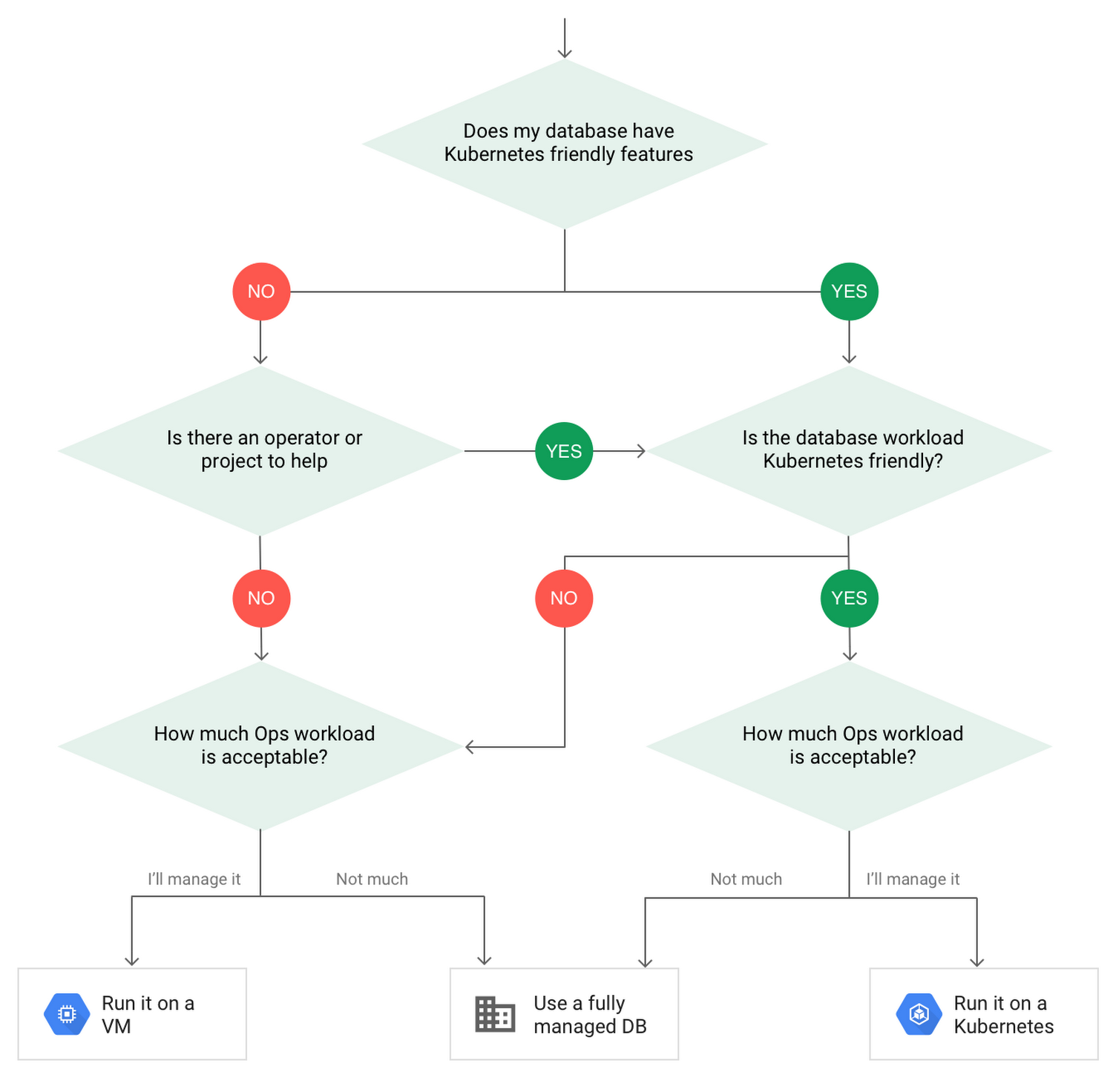
When choosing to go down the Kubernetes route, think about what database you will be running, and how well it will work given the trade-offs previously discussed.
Since pods are mortal, the likelihood of failover events is higher than a traditionally hosted or fully managed database. It will be easier to run a database on Kubernetes if it includes concepts like sharding, failover elections and replication built into its DNA (for example, ElasticSearch, Cassandra, or MongoDB). Some open source projects provide custom resources and operators to help with managing the database.
Next, consider the function that database is performing in the context of your application and business. Databases that are storing more transient and caching layers are better fits for Kubernetes. Data layers of that type typically have more resilience built into the applications, making for a better overall experience.
Finally, be sure you understand the replication modes available in the database. Asynchronous modes of replication leave room for data loss, because transactions might be committed to the primary database but not to the secondary database(s). So, be sure to understand whether you might incur data loss, and how much of that is acceptable in the context of your application.
After evaluating all of those considerations, you’ll end up with a decision tree looking something like this:
How to deploy a database on Kubernetes
Now, let’s dive into more details on how to deploy a database on Kubernetes using StatefulSets.
With a StatefulSet, your data can be stored on persistent volumes, decoupling the database application from the persistent storage, so when a pod (such as the database application) is recreated, all the data is still there.
Additionally, when a pod is recreated in a StatefulSet, it keeps the same name, so you have a consistent endpoint to connect to. Persistent data and consistent naming are two of the largest benefits of StatefulSets. You can check out the Kubernetes documentation for more details.
If you need to run a database that doesn’t perfectly fit the model of a Kubernetes-friendly database (such as MySQL or PostgreSQL), consider using Kubernetes Operators or projects that wrap those database with additional features. Operators will help you spin up those databases and perform database maintenance tasks like backups and replication. For MySQL in particular, take a look at the Oracle MySQL Operator and Crunchy Data for PostgreSQL.
Operators use custom resources and controllers to expose application-specific operations through the Kubernetes API. For example, to perform a backup using Crunchy Data, simply execute pgo backup [cluster_name]. To add a Postgres replica, use pgo scale cluster [cluster_name].
There are some other projects out there that you might explore, such as Patroni for PostgreSQL. These projects use Operators, but go one step further. They’ve built many tools around their respective databases to aid their operation inside of Kubernetes. They may include additional features like sharding, leader election, and failover functionality needed to successfully deploy MySQL or PostgreSQL in Kubernetes.
While running a database in Kubernetes is gaining traction, it is still far from an exact science. There is a lot of work being done in this area, so keep an eye out as technologies and tools evolve toward making running databases in Kubernetes much more the norm.
When you’re ready to get started, check out GCP Marketplace for easy-to-deploy SaaS, VM, and containerized database solutions and operators that can be deployed to GCP or Kubernetes clusters anywhere.
More Relevant Stories for Your Company

BigQuery ML for Sentiment Analysis: How to Make the Most of Your Data
Introduction We recently announced BigQuery support for sparse features which help users to store and process the sparse features efficiently while working with them. That functionality enables users to represent sparse tensors and train machine learning models directly in the BigQuery environment. Being able to represent sparse tensors is a

Quick Tips to Get the Most Out of Cloud Spanner
Today, IT Admins and DBAs are inundated with thankless tasks. But they no longer have to deal with that. With Cloud Spanner, they can focus on value-add and innovation instead of maintenance. Creating or scaling a globally replicated database for mission-critical apps now takes a handful of clicks. Industry-leading high-availability

Creating and Using Storage Buckets for Your Data Needs
So, you want to store objects on the cloud? But you're really new to Google Cloud or Cloud Storage and would like someone to walk you through the process step by step? Today is your lucky day! I will help you understand the big steps involved in setting up and



An Overview of Google’s Data Cloud
Data access, management and privacy has been at the center of priorities for enterprises that are aiming to be more agile, reliable and data-driven. Google Cloud's technology innovations spanning products like BigQuery, Spanner, Looker and VertexAI help organizations navigate the complexities related to siloed data in large volumes sprawled across
