





How to Pick a Database that is Suitable for Your Application

7015
Of your peers have already read this article.
2:30 Minutes
The most insightful time you'll spend today!
Picking the right database for your application is not easy. The choice depends heavily on your use case—transactional processing, analytical processing, in-memory database, and so on—but it also depends on other factors. This post covers the different database options available within Google Cloud across relational (SQL) and non-relational (NoSQL) databases and explains which use cases are best suited for each database option.

Relational databases
In relational databases information is stored in tables, rows and columns, which typically works best for structured data. As a result they are used for applications in which the structure of the data does not change often. SQL (Structured Query Language) is used when interacting with most relational databases. They offer ACID consistency mode for the data, which means:
- Atomic: All operations in a transaction succeed or the operation is rolled back.
- Consistent: On the completion of a transaction, the database is structurally sound.
- Isolated: Transactions do not contend with one another. Contentious access to data is moderated by the database so that transactions appear to run sequentially.
- Durable: The results of applying a transaction are permanent, even in the presence of failures.
Because of these properties, relational databases are used in applications that require high accuracy and for transactional queries such as financial and retail transactions. For example: In banking when a customer makes a funds transfer request, you want to make sure the transaction is possible and it actually happens on the most up-to-date account balance, in this case an error or resubmit request is likely fine.
There are three relational database options in Google Cloud: Cloud SQL, Cloud Spanner, and Bare Metal Solution.
Cloud SQL: Provides managed MySQL, PostgreSQL and SQL Server databases on Google Cloud. It reduces maintenance cost and automates database provisioning, storage capacity management, back ups, and out-of-the-box high availability and disaster recovery/failover. For these reasons it is best for general-purpose web frameworks, CRM, ERP, SaaS and e-commerce applications.
Cloud Spanner: Cloud Spanner is an enterprise-grade, globally-distributed, and strongly-consistent database that offers up to 99.999% availability, built specifically to combine the benefits of relational database structure with non-relational horizontal scale. It is a unique database that combines ACID transactions, SQL queries, and relational structure with the scalability that you typically associate with non-relational or NoSQL databases. As a result, Spanner is best used for applications such as gaming, payment solutions, global financial ledgers, retail banking and inventory management that require ability to scale limitlessly with strong-consistency and high-availability.
Bare Metal Solution: Provides hardware to run specialized workloads with low latency on Google Cloud. This is specifically useful if there is an Oracle database that you want to lift and shift into Google Cloud. This enables data center retirements and paves a path to modernize legacy applications.
Non-relational databases
Non-relational databases (or NoSQL databases) store compex, unstructured data in a non-tabular form such as documents. Non-relational databases are often used when large quantities of complex and diverse data need to be organized. Unlike relational databases, they perform faster because a query doesn’t have to access several tables to deliver an answer, making them ideal for storing data that may change frequently or for applications that handle many different kinds of data.
For example, an apparel store might have a database in which shirts have their own document containing all of their information, including size, brand, and color with room for adding more parameters later such as sleeve size, collars, and so on.
Qualities that make NoSQL databases fast:
- Eventual consistency: stores usually exhibit consistency at some later point (e.g., lazily at read time)
- Horizontal scaling, usually using hashed distributions
- Typically, they are optimized for a specific workload pattern (i.e., key-value, graph, wide-column)
- Typically, they don’t support cross shard transactions or flexible isolation modes.
Because of these properties, non-relational databases are used in applications that require large scale, reliability, availability, and frequent data changes.They can easily scale horizontally by adding more servers, unlike some relational databases, which scale vertically by increasing the machine size as the data grows. Although, some relations databases such as Cloud Spanner support scale-out and strict consistency.
Non-relational databases can store a variety of unstructured data such as documents, key-value, graphs, wide columns, and more. Here are your non-relational database options in Google Cloud:
- Document databases: Store information as documents (in formats such as JSON and XML). For example: Firestore
- Key-value stores: Group associated data in collections with records that are identified with unique keys for easy retrieval. Key-value stores have just enough structure to mirror the value of relational databases while still preserving the benefits of NoSQL. For example: Datastore, Bigtable, Memorystore
- In-memory database: Purpose-built database that relies primarily on memory for data storage. These are designed to attain minimal response time by eliminating the need to access disks. They are ideal for applications that require microsecond response times and can have large spikes in traffic. For example: Memorystore
- Wide-column databases: Use the tabular format but allow a wide variance in how data is named and formatted in each row, even in the same table. They have some basic structure while preserving a lot of flexibility. For example: Bigtable
- Graph databases: Use graph structures to define the relationships between stored data points; useful for identifying patterns in unstructured and semi-structured information. For example: JanusGraph
There are three non-relational databases in Google Cloud:
- Firestore: Is a serverless document database which scales on demand and acts as a backend-as-a-service. It is DBaaS that increases the speed of building applications. It is perfect for all general purpose uses cases such as ecommerce, gaming, IoT and real time dashboards. With Firestore users can interact with and collaborate on live and offline data making it great for real-time application and mobile apps.
- Cloud Bigtable: Cloud Bigtable is a sparsely populated table that can scale to billions of rows and thousands of columns, enabling you to store terabytes or even petabytes of data. It is ideal for storing very large amounts of single-keyed data with very low latency. It supports high read and write throughput at sub-millisecond latency, and it is an ideal data source for MapReduce operations. It also supports the open-source HBase API standard to easily integrate with the Apache ecosystem including HBase, Beam, Hadoop and Spark along with Google Cloud ecosystem.
- Memorystore: Memorystore is a fully managed in-memory data store service for Redis and Memcached at Google Cloud. It is best for in-memory and transient data stores and automates the complex tasks of provisioning, replication, failover, and patching so you can spend more time coding. Because it offers extremely low latency and high performance, Memorystore is great for web and mobile, gaming, leaderboard, social, chat, and news feed applications.
Conclusion
Choosing a relational or a non-relational database largely depends on the use case. Broadly, if your application requires ACID transactions and your data structure is not going to change much, select a relational database.
In Google Cloud use Cloud SQL for any general-purpose SQL database and Cloud Spanner for large-scale globally scalable, strongly consistent use cases. In general, if your data structure may change later and if scale and availability is a bigger requirement than consistency then a non-relational database is a preferable choice. Google Cloud offers Firestore, Memorystore, and Cloud Bigtable to support a variety of use cases across the document, key-value, and wide column database spectrum.
For more comparison resources on each database check out the overview. For more hands-on experience with Bigtable, check out our on-demand training here and learn about migrating databases to managed services check out this whitepaper.
https://youtube.com/watch?v=2TZXSnCTd7E%3Fenablejsapi%3D1%26
For more #GCPSketchnote, follow the GitHub repo. For similar cloud content follow me on Twitter @pvergadia and keep an eye out on thecloudgirl.dev.
3289
Of your peers have already watched this video.
24:30 Minutes
The most insightful time you'll spend today!
Modernizing 100-Year Old Retail Chain with Anthos
H-E-B, like many enterprises, was moving away from legacy mainframes in favor of microservices and public cloud infrastructure. With hundreds of applications powering their 100+ year-old business, H-E-B needed to be confident that the platform they are building will provide them the agility and security to continue to innovate for their customers.
See how the H-E-B engineering team started breaking down their Curbside and Home Delivery monoliths into microservices, why they chose to make Kubernetes, and why they’re leveraging Anthos as a hybrid cloud platform.
The Latest in Spring Cloud GCP: Upgrading the Sample Bank of Anthos App

1392
Of your peers have already read this article.
3:30 Minutes
The most insightful time you'll spend today!
We’re excited to announce that Spring Cloud GCP version 4.0 is now generally available! In this post, we’ll be describing what the new major version has to offer, and demonstrating the process of using the migration guide on one of our reference architectures, Bank of Anthos.
What’s new?
With this release, Spring Cloud GCP officially supports Spring Boot 3.x. However, this migration involves a number of breaking changes as outlined in the migration guide. The full list of changes made is available on Github, but the one of the most significant differences is that Java 17 is now a minimum requirement.
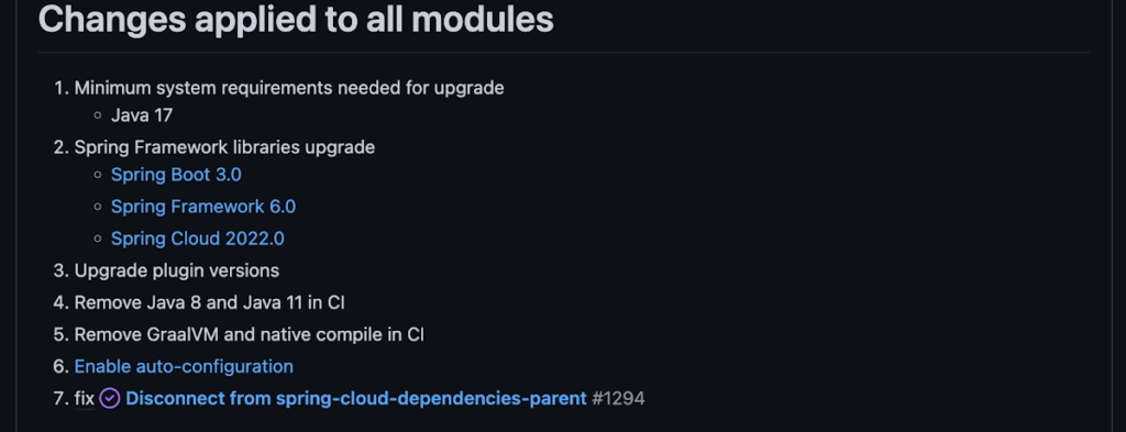
Another notable feature of this release is the addition of starter artifacts – Spring Boot starters for Google Cloud – that provide dependencies and auto-configurations for 80+ Google Client libraries. Just as the name suggests, these starters can serve as helpful starting points when working with a new client library. For now, they’re in preview.
These starters are not included in the BOM by default and need to be added as a dependency to your project before they can be used. For example, if you wanted to get started with Cloud Text-to-Speech, you would include the following:
<dependency>
    <groupId>com.google.cloud</groupId>
    <artifactId>google-cloud-texttospeech-spring-starter</artifactId>
    <version>4.0.0-preview</version>
  </dependency>
The upgrade process
We prepared a migration guide to help answer any questions involved with moving from 3.x to 4.x. Let’s follow those instructions to migrate Bank of Anthos.
We’ll start by cloning and building the application before the upgrade, according to the quickstart and development guide:
PROJECT_ID=<YOUR-PROJECT-ID>
gcloud services enable container --project ${PROJECT_ID}

git clone https://github.com/GoogleCloudPlatform/bank-of-anthos.git
cd bank-of-anthos/

gcloud services enable container.googleapis.com monitoring.googleapis.com \
  --project ${PROJECT_ID}

REGION=us-central1
gcloud container clusters create-auto bank-of-anthos \
  --project=${PROJECT_ID} --region=${REGION}

gcloud container clusters get-credentials bank-of-anthos \
  --project=${PROJECT_ID} --region=${REGION}

skaffold run --default-repo=gcr.io/${PROJECT_ID}/bank-of-anthos
At the end of this, you should see a “deployment stabilized” message:
Deployments stabilized in 9.657 secondsWith the environment set up for development, we’re ready to move on to the actual migration. The migration is already complete at time of writing, but here’s the full list of changes made:
- We began by checking the current Java, Spring Boot and Spring Cloud GCP versions.
- Our Java version is okay, but the other two are out of date, and will need to be updated.
We can also add the Spring Cloud GCP BOM to manage our versions going forward while we’re here.
- Our Java version is okay, but the other two are out of date, and will need to be updated.
- Then, in no particular order, we can make the following code changes:
- Remove the explicit type declarations from our ResponseEntity instantiations.
- Replace all javax.* imports with Jakarta.* counterparts, since Spring 3.0 makes use of Jakarta EE 9.0
With those changes in place, the app is upgraded and ready to re-deploy!
Live example
For a finished example of this migration, check out the Bank of Anthos repository on Github. It’s an excellent sample application that showcases a polyglot Java & Python app, served on Kubernetes and Google Cloud. All CI/CD and configurations are open source, so it may be instructive as you approach this migration.
Thanks for reading, and feel free to provide comments or feedback on Twitter, or in the issues section of the repository.
10147
Of your peers have already watched this video.
1:00 Minutes
The most insightful time you'll spend today!
Predict User Churn on Gaming Apps with Google Analytics Data using BigQuery ML
User retention can be a major challenge for mobile game developers. According to the Mobile Gaming Industry Analysis in 2019, most mobile games only see a 25% retention rate for users after the first day. To retain a larger percentage of users after their first use of an app, developers can take steps to motivate and incentivize certain users to return. But to do so, developers need to identify the propensity of any specific user returning after the first 24 hours.
In this blog post, we will discuss how you can use BigQuery ML to run propensity models on Google Analytics 4 data from your gaming app to determine the likelihood of specific users returning to your app.
You can also use the same end-to-end solution approach in other types of apps using Google Analytics for Firebase as well as apps and websites using Google Analytics 4. To try out the steps in this blogpost or to implement the solution for your own data, you can use this Jupyter Notebook.
Using this blog post and the accompanying Jupyter Notebook, you’ll learn how to:
- Explore the BigQuery export dataset for Google Analytics 4
- Prepare the training data using demographic and behavioural attributes
- Train propensity models using BigQuery ML
- Evaluate BigQuery ML models
- Make predictions using the BigQuery ML models
- Implement model insights in practical implementations
Google Analytics 4 (GA4) properties unify app and website measurement on a single platform and are now default in Google Analytics. Any business that wants to measure their website, app, or both, can use GA4 for a more complete view of how customers engage with their business. With the launch of Google Analytics 4, BigQuery export of Google Analytics data is now available to all users. If you are already using a Google Analytics 4 property, you can follow this guide to set up exporting your GA data to BigQuery.
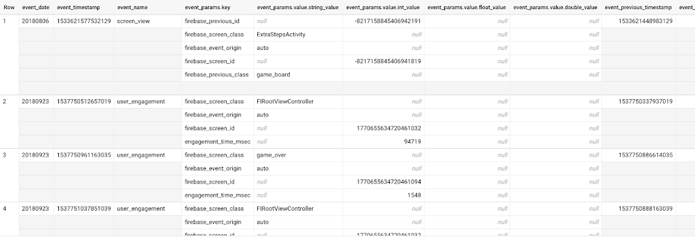
Once you have set up the BigQuery export, you can explore the data in BigQuery. Google Analytics 4 uses an event-based measurement model. Each row in the data is an event with additional parameters and properties. The Schema for BigQuery Export can help you to understand the structure of the data.
In this blogpost, we use the public sample export data from an actual mobile game app called “Flood It!” (Android, iOS) to build a churn prediction model. But you can use data from your own app or website.
Here’s what the data looks like. Each row in the dataset is a unique event, which can contain nested fields for event parameters.
SELECT *FROM `firebase-public-project.analytics_153293282.events_*`TABLESAMPLE SYSTEM (1 PERCENT)
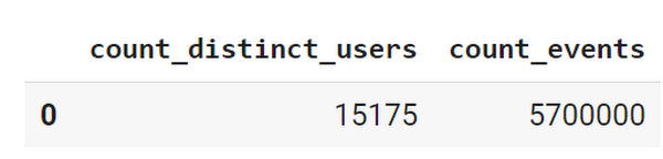
This dataset contains 5.7M events from over 15k users.
SELECTCOUNT(DISTINCT user_pseudo_id) as count_distinct_users,COUNT(event_timestamp) as count_eventsFROM`firebase-public-project.analytics_153293282.events_*
Our goal is to use BigQuery ML on the sample app dataset to predict propensity to user churn or not churn based on users’ demographics and activities within the first 24 hours of app installation.
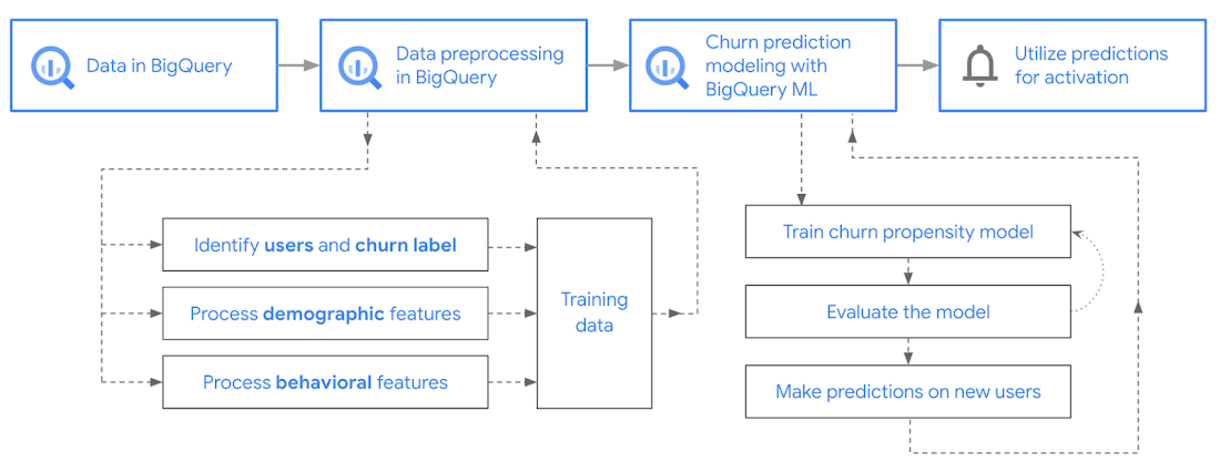
In the following sections, we’ll cover how to:
- Pre-process the raw event data from GA4
- Identify users & the label feature
- Process demographic features
- Process behavioral features
- Train classification model using BigQuery ML
- Evaluate the model using BigQueryML
- Make predictions using BigQuery ML
- Utilize predictions for activation
Pre-process the raw event data
You cannot simply use raw event data to train a machine learning model as it would not be in the right shape and format to use as training data. So in this section, we’ll go through how to pre-process the raw data into an appropriate format to use as training data for classification models.
This is what the training data should look like for our use case at the end of this section:
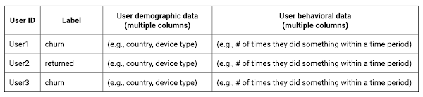
Notice that in this training data, each row represents a unique user with a distinct user ID (user_pseudo_id).
Identify users & the label feature
We first filtered the dataset to remove users who were unlikely to return the app anyway. We defined these ‘bounced’ users as ones who spent less than 10 mins with the app. Then we labeled all remaining users:
- churned: No event data for the user after 24 hours of first engaging with the app.
- returned: The user has at least one event record after 24 hours of first engaging with the app.
For your use case, you can have a different definition of bounce and churning. Also you can even try to predict something else other than churning, e.g.:
- whether a user is likely to spend money on in-game currency
- likelihood of completing n-number of game levels
- likelihood of spending n amount of time in-game etc.
In such cases, label each record accordingly so that whatever you are trying to predict can be identified from the label column.
From our dataset, we found that ~41% users (5,557) bounced. However, from the remaining users (8,031), ~23% (1,883) churned after 24 hours:
SELECTbounced,churned,COUNT(churned) as count_usersFROMbqmlga4.returningusersGROUP BY 1,2ORDER BY bounced
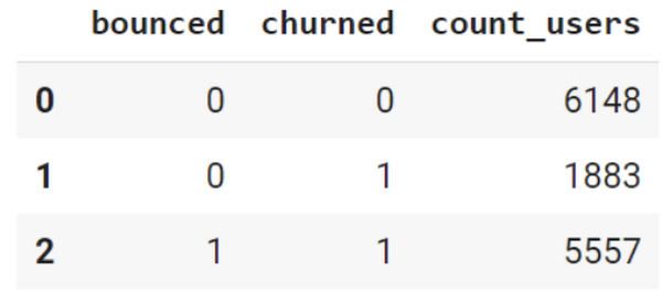
To create these bounced and churned columns, we used the following snippet of SQL code.
...#churned = 1 if last_touch within 24 hr of app installation, else 0IF (user_last_engagement < TIMESTAMP_ADD(user_first_engagement,INTERVAL 24 HOUR),1,0 ) AS churned,#bounced = 1 if last_touch within 10 min, else 0IF (user_last_engagement <= TIMESTAMP_ADD(user_first_engagement,INTERVAL 10 MINUTE),1,0 ) AS bounced,...
You can view the Jupyter Notebook for the full query used for materializing the bounced and churned labels.
Process demographic features
Next, we added features both for demographic data and for behavioral data spanning across multiple columns. Having a combination of both demographic data and behavioral data helps to create a more predictive model.
We used the following fields for each user as demographic features:
geo.countrydevice.operating_systemdevice.language
A user might have multiple unique values in these fields — for example if a user uses the app from two different devices. To simplify, we used the values from the very first user engagement event.
CREATE OR REPLACE VIEW bqmlga4.user_demographics AS (WITH first_values AS (SELECTuser_pseudo_id,geo.country as country,device.operating_system as operating_system,device.language as language,ROW_NUMBER() OVER (PARTITION BY user_pseudo_id ORDER BY event_timestamp DESC) AS row_numFROM `firebase-public-project.analytics_153293282.events_*`WHERE event_name="user_engagement")SELECT * EXCEPT (row_num)FROM first_valuesWHERE row_num = 1 #first engagement);
Process behavioral features
There is additional demographic information present in the GA4 export dataset, e.g. app_info, device, event_params, geo etc. You may also send demographic information to Google Analytics through each hit via user_properties. Furthermore, if you have first-party data on your own system, you can join that with the GA4 export data based on user_ids.
To extract user behavior from the data, we looked into the user’s activities within the first 24 hours of first user engagement. In addition to the events automatically collected by Google Analytics, there are also the recommended events for games that can be explored to analyze user behavior. For our use case, to predict user churn, we counted the number of times the follow events were collected for a user within 24 hours of first user engagement:
user_engagementlevel_start_quickplaylevel_end_quickplaylevel_complete_quickplaylevel_reset_quickplaypost_scorespend_virtual_currencyad_rewardchallenge_a_friendcompleted_5_levelsuse_extra_steps
The following query shows how these features were calculated:
WITHevents_first24hr AS (SELECTe.*FROM`firebase-public-project.analytics_153293282.events_*` eJOINbqmlga4.returningusers rONe.user_pseudo_id = r.user_pseudo_idWHERETIMESTAMP_MICROS(e.event_timestamp) <= r.ts_24hr_after_first_engagement)SELECTuser_pseudo_id,SUM(IF(event_name = 'user_engagement', 1, 0)) AS cnt_user_engagement,# ... repeated for all behavior data ...SUM(IF(event_name = 'use_extra_steps', 1, 0)) AS cnt_use_extra_steps,FROMevents_first24hrGROUP BY1
View the notebook for the query used to aggregate and extract the behavioral data. You can use different sets of events for your use case. To view the complete list of events, use the following query:
SELECTevent_name,COUNT(event_name) as event_countFROM`firebase-public-project.analytics_153293282.events_*`GROUP BY 1ORDER BYevent_count DESC
After this we combined the features to ensure our training dataset reflects the intended structure. We had the following columns in our table:
- User ID:
user_pseudo_id
- Label:
churned
- Demographic features
countrydevice_osdevice_language
- Behavioral features
cnt_user_engagementcnt_level_start_quickplaycnt_level_end_quickplaycnt_level_complete_quickplaycnt_level_reset_quickplaycnt_post_scorecnt_spend_virtual_currencycnt_ad_rewardcnt_challenge_a_friendcnt_completed_5_levelscnt_use_extra_stepsuser_first_engagement
At this point, the dataset was ready to train the classification machine learning model in BigQuery ML. Once trained, the model will output a propensity score between churn (churned=1) or return (churned=0) indicating the probability of a user churning based on the training data.
Train classification model
When using the CREATE MODEL statement, BigQuery ML automatically splits the data between training and test. Thus the model can be evaluated immediately after training (see the documentation for more information).
For the ML model, we can choose among the following classification algorithms where each type has its own pros and cons:
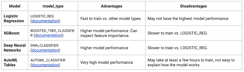
Often logistic regression is used as a starting point because it is the fastest to train. The query below shows how we trained the logistic regression classification models in BigQuery ML.
CREATE OR REPLACE MODEL bqmlga4.churn_logregTRANSFORM(EXTRACT(MONTH from user_first_engagement) as month,EXTRACT(DAYOFYEAR from user_first_engagement) as julianday,EXTRACT(DAYOFWEEK from user_first_engagement) as dayofweek,EXTRACT(HOUR from user_first_engagement) as hour,* EXCEPT(user_first_engagement, user_pseudo_id))OPTIONS(MODEL_TYPE="LOGISTIC_REG",INPUT_LABEL_COLS=["churned"]) ASSELECT*FROMbqmlga4.train
We extracted month, julianday, and dayofweek from datetimes/timestamps as one simple example of additional feature preprocessing before training. Using TRANSFORM() in your CREATE MODEL query allows the model to remember the extracted values. Thus, when making predictions using the model later on, these values won’t have to be extracted again. View the notebook for the example queries to train other types of models (XGBoost, deep neural network, AutoML Tables).
Evaluate model
Once the model finished training, we ran ML.EVALUATE to generate precision, recall, accuracy and f1_score for the model:
SELECT*FROMML.EVALUATE(MODEL bqmlga4.churn_logreg)

The optional THRESHOLD parameter can be used to modify the default classification threshold of 0.5. For more information on these metrics, you can read through the definitions on precision and recall, accuracy, f1-score, log_loss and roc_auc. Comparing the resulting evaluation metrics can help to decide among multiple models.Furthermore, we used a confusion matrix to inspect how well the model predicted the labels, compared to the actual labels. The confusion matrix is created using the default threshold of 0.5, which you may want to adjust to optimize for recall, precision, or a balance (more information here).
SELECTexpected_label,_0 AS predicted_0,_1 AS predicted_1FROMML.CONFUSION_MATRIX(MODEL bqmlga4.churn_logreg)
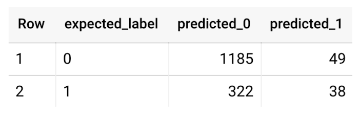
This table can be interpreted in the following way:

Make predictions using BigQuery ML
Once the ideal model was available, we ran ML.PREDICT to make predictions. For propensity modeling, the most important output is the probability of a behavior occurring. The following query returns the probability that the user will return after 24 hrs. The higher the probability and closer it is to 1, the more likely the user is predicted to return, and the closer it is to 0, the more likely the user is predicted to churn.
SELECTuser_pseudo_id,returned,predicted_returned,predicted_returned_probs[OFFSET(0)].prob as probability_returnedFROMML.PREDICT(MODEL bqmlga4.churn_logreg,(SELECT * FROM bqmlga4.train)) #can be replaced with a proper test dataset
Utilize predictions for activation
Once the model predictions are available for your users, you can activate this insight in different ways. In our analysis, we used user_pseudo_id as the user identifier. However, ideally, your app should send back the user_id from your app to Google Analytics. In addition to using first-party data for model predictions, this will also let you join back the predictions from the model into your own data.
- You can import the model predictions back into Google Analytics as a user attribute. This can be done using the Data Import feature for Google Analytics 4. Based on the prediction values you can Create and edit audiences and also do Audience targeting. For example, an audience can be users with prediction probability between 0.4 and 0.7, to represent users who are predicted to be “on the fence” between churning and returning.
- For Firebase Apps, you can use the Import segments feature. You can tailor user experience by targeting your identified users through Firebase services such as Remote Config, Cloud Messaging, and In-App Messaging. This will involve importing the segment data from BigQuery into Firebase. After that you can send notifications to the users, configure the app for them, or follow the user journeys across devices.
- Run targeted marketing campaigns via CRMs like Salesforce, e.g. send out reminder emails.
You can find all of the code used in this blogpost in the Github repository:
What’s next?
Continuous model evaluation and re-training
As you collect more data from your users, you may want to regularly evaluate your model on fresh data and re-train the model if you notice that the model quality is decaying.
Continuous evaluation—the process of ensuring a production machine learning model is still performing well on new data—is an essential part in any ML workflow. Performing continuous evaluation can help you catch model drift, a phenomenon that occurs when the data used to train your model no longer reflects the current environment.
To learn more about how to do continuous model evaluation and re-train models, you can read the blogpost: Continuous model evaluation with BigQuery ML, Stored Procedures, and Cloud Scheduler
More resources
If you’d like to learn more about any of the topics covered in this post, check out these resources:
- BigQuery export of Google Analytics data
- BigQuery ML quickstart
- Events automatically collected by Google Analytics 4
- Qwiklabs: Create ML models with BigQuery ML
Or learn more about how you can use BigQuery ML to easily build other machine learning solutions:
- How to build demand forecasting models with BigQuery ML
- How to build a recommendation system on e-commerce data using BigQuery ML
Let us know what you thought of this post, and if you have topics you’d like to see covered in the future! You can find us on Twitter at @polonglin and @_mkazi_.Thanks to reviewers: Abhishek Kashyap, Breen Baker, David Sabater Dinter.
How to Build A Basic Image Search Utility for Natural Language Queries

4684
Of your peers have already read this article.
6:00 Minutes
The most insightful time you'll spend today!
This post shows how to build an image search utility using natural language queries. Our aim is to use different GCP services to demonstrate this. At the core of our project is OpenAI’s CLIP model. It makes use of two encoders – one for images and one for texts. Each encoder is trained to learn representations such that similar images and text embeddings are projected as close as possible.
We will first create a Flask-based REST API capable of handling natural language queries and matching them against relevant images. We will then demonstrate the use of the API through a Flutter-based web and mobile application. Figure 1 shows how our final application would look like:
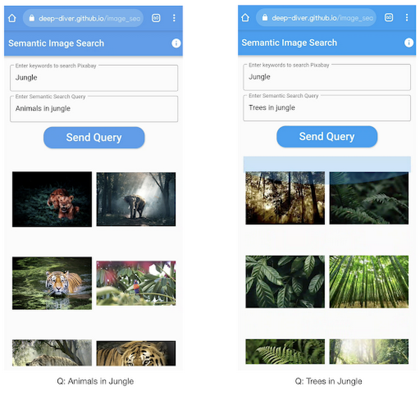
All the code shown in this post is available as a GitHub repository. Let’s dive in.
Application at a high-level
Our application will take two queries from the user:
- Tag or keyword query. This is needed in order to pull a set of images of interest from Pixabay. You can use any other image repositories for this purpose. But we found Pixabay’s API to be easier to work with. We will cache these images to optimize the user experience. Suppose we wanted to find images that are similar to this query: “horses amidst flowers”. For this, we’d first pull in a few “horse” images and then run another utility to find out the images that best match our query.
- Longer or semantic query that we will use to retrieve the images from the pool created in the step above. These images should be semantically similar to this query.
Note: Instead of two queries, we could have only taken a single long query and run named-entity extraction to determine the most likely important keywords to run the initial search with. For this post, we won’t be using this approach.
Figure 2 below depicts the architecture design of our application and the technical stack used for each of the components.
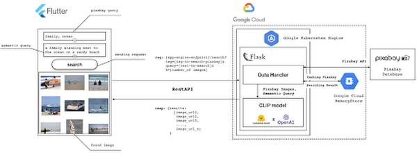
Figure 2 also presents the core logic of the API we will develop in bits and pieces in this post. We will deploy this API on a Kubernetes cluster using the Google Kubernetes Engine (GKE). The following presents a brief directory structure of our application code-base:
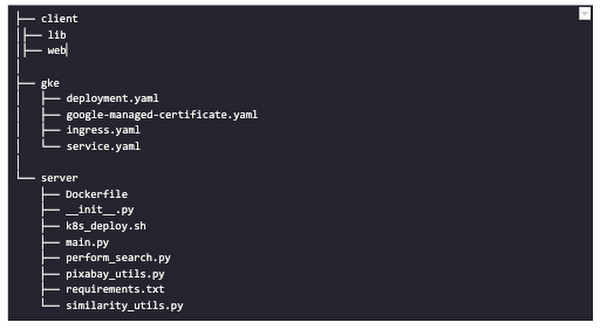
Next, we will walk through the code and other related components for building our image search API. For various machine learning-related utilities, we will be using PyTorch.
Building the backend API with Flask
First, we’d need to fetch a set of images with respect to user-provided tags/keywords before performing the natural language image search. The utility below from the pixabay_utils.py script can do this for us:
def fetch_images_tag(pixabay_search_keyword, num_images):"""Fetches images from Pixabay w.r.t a keyword.:param pixabay_search_keyword: Keyword to perform the search on Pixabay.:param num_images: Number of images to retrieve.:return: List of PIL images.:return: List of image URLs."""query = (PIXABAY_API+ "&q="+ pixabay_search_keyword.lower()+ "&image_type=photo&safesearch=true&per_page="+ str(num_images))response = requests.get(query)output = response.json()all_images = []all_image_urls = []for each in output["hits"]:imageurl = each["webformatURL"]response = requests.get(imageurl)image = Image.open(BytesIO(response.content)).convert("RGB")all_images.append(image)all_image_urls.append(imageurl)return (all_images, all_image_urls)
Note that all the API utilities are logging relevant information. But for brevity, we have omitted the lines of code responsible for that. Next, we will see how to invoke the CLIP model and select the images that would best match a given query semantically. For this, we’ll be using Hugging Face, an easy-to-use Python library offering state-of-the-art NLP capabilities. We’ll collate all the logic related to this search inside a SimilarityUtil class:
class SimilarityUtil:def __init__(self):self.model = CLIPModel.from_pretrained(CLIP_MODEL)self.processor = CLIPProcessor.from_pretrained(CLIP_PREPROCESSOR)self.device = "cuda" if torch.cuda.is_available() else "cpu"def perform_sim_search(self, images, query_phrase, top_k=3):"""Performs similarity search between the images and query.:param images: A list of PIL images initially retrieved withrespect to some entity e.g. Tiger.:param query_phrase: A list containing a single text query,e.g. "Tiger drinking water".:param top_k: Number of top images to return from `images`.:return: Top-k indices matching the query semantically andtheir similarity scores."""model = self.model.to(self.device)# Obtain the text-image similarity scoreswith torch.no_grad():inputs = self.processor(text=[query_phrase], images=images, return_tensors="pt", padding=True)inputs = inputs.to(self.device)outputs = model(**inputs)# Image-text similarity scoreslogits_per_image = outputs.logits_per_image.cpu()(top_indices, top_scores) = self.sort_scores(logits_per_image, top_k)return (top_indices, top_scores)def sort_scores(self, scores, top_k):"""Sorts the scores in a descending manner.:param scores: Scores to sort through.:param top_k: Number of top scores to return.:return: Top-k scores and their indices."""values, indices = scores.squeeze().topk(top_k)top_indices, top_scores = [], []for score, index in zip(values, indices):top_indices.append(int(index.numpy()))score = score.numpy().tolist()top_scores.append(round(score, 3))return (top_indices, top_scores)
CLIP_MODEL uses a ViT-base model to encode the images for generating meaningful embeddings with respect to the provided query. The text-based query is also encoded using A Transformers-based model for generating the embeddings. These two embeddings are matched with one another during inference. To know more about the particular methods we are using for the CLIP model please refer to this documentation from Hugging Face.
In the code above, we are first invoking the CLIP model with images and the natural language query. This gives us a vector (logits_per_image) that contains the similarity scores between each of the images and the query. We then sort the vector in a descending manner. Note that we are initializing the CLIP model while instantiating the SimilarityUtil to save us the model loading time. This is the meat of our application and we have tackled it already. If you want to interact with this utility in a live manner you can check out this Colab Notebook.
Now, we need to collate our utilities for fetching images from Pixabay and for performing the natural language image search inside a single script – perform_search.py. Following is the main class of that script:
class Searcher:def __init__(self):self.similarity_model = SimilarityUtil()def get_similar_images(self, keyword, semantic_query, pixabay_max, top_k):"""Finds semantically similar images.:param keyword: Keyword to search with on Pixabay.:param semantic_query: Query to find semantically similar images retrieved from Pixabay.:param pixabay_max: Number of maximum images to retrieve from Pixabay.:param top_k: Top-k images to return.:return: Tuple of top_k URLs and the similarity scores of the images present inside the URLs."""images_redis_key = keyword + "_images"urls_redis_key = keyword + "_urls"if redis_client.exists(images_redis_key) and redis_client.exists(urls_redis_key):keyword_images = redis_client.get(images_redis_key)keyword_image_urls = redis_client.get(urls_redis_key)else:(keyword_images, keyword_image_urls) = fetch_images_tag(keyword, pixabay_max)redis_client.set(images_redis_key, keyword_images)redis_client.set(urls_redis_key, keyword_image_urls)(top_indices, top_scores) = self.similarity_model.perform_sim_search(keyword_images, semantic_query, top_k)top_urls = [keyword_image_urls[index] for index in top_indices]return (top_urls, top_scores)
Here, we are just calling the utilities we had previously developed to return the URLs of the most similar images and their scores. What is even more important here is the caching capability. For that, we combined GCP’s MemoryStore and a Python library called direct-redis. More on setting up MemoryStore later.
MemoryStore provides a fully managed and low-cost platform for hosting Redis instances. Redis databases are in memory and light-weight making them an ideal candidate for caching. In the code above, we are caching the images fetched from Pixabay and their URLs. So, in the event of a cache hit, we won’t need to call the CLIP model and this will tremendously improve the response time of our API.
Other options for caching
We can cache other elements of our application. For example, the natural language query. When searching through the cached entries to determine if it’s a cache hit, we can compare two queries for semantic similarity and return results accordingly.
Consider that a user had entered the following natural language query: “mountains with dark skies”. After performing the search, we’d cache the embeddings of this query. Now, consider that another user entered another query: “mountains with gloomy ambiance”. We’d compute its embeddings and run a similarity search with the cached embeddings. We’d then compare the similarity scores with respect to a threshold and parse the most similar queries and their corresponding results. In case of a cache miss, we’d just call the image search utilities we developed above.
When working on real-time applications we often need to consider these different aspects and decide what enhances the user experience and maximizes business at the same time.
All that’s left now for the backend is our Flask application – main.py:
@app.route("/search", methods=["GET"])def get_images():tag = request.args.get("t").lower()query = request.args.get("s_query").lower()top_k = request.args.get("k")(top_urls, top_scores) = searcher.get_similar_images(tag, query, MAX_PIXABAY_SEARCH, int(top_k))return jsonify({"top_urls": top_urls, "top_scores": top_scores})
Here we are first parsing the query parameters from the request payload of our search API. We are then just calling the appropriate function from perform_search.py to handle the request. This Flask application is also capable of handling CORS. We do this via the flask_cors library:
cors = CORS(app,resources={r"/search/*": {"origin": "*"},r"/test/*": {"origin": "*"},},)
And this is it! Our API is now ready for deployment.
Deployment with Compute Engine and GKE
The reason why we wanted to deploy our API on Kubernetes is because of the flexibility Kubernetes offers for managing deployments. When operating at scale, auto scalability and load balancing are very important. With the comes the requirement of security — we’d not want to expose the utilities for interacting with any internal services such as databases. With Kubernetes, we can achieve all these easily and efficiently.
GKE provides secured and fully managed functionalities for operationalizing Kubernetes clusters. Here are the steps to deploy the API on GKE at a glance:
- We first build a Docker image for our API and then push it to the Google Container Registry (GCR).
- We then create a Kubernetes cluster on GKE and initialize a deployment.
- We then add scalability options.
- If any public exposure is needed for the API, we then tackle it.
We can assimilate all the above into a shell script – k8s_deploy.sh:
## Docker build and push ### We are inside the `server` directorydocker build -t gcr.io/${PROJECT_ID}/search_service .docker push gcr.io/${PROJECT_ID}/search_service## Deploy on a GKE cluster ### Configure the Docker command-line tool to authenticate to Container Registrygcloud auth configure-docker# Create a Kubernetes clustergcloud container clusters create image-search-nlp# Create a deploymentkubectl create deployment clip-search --image=gcr.io/${PROJECT_ID}/search_service# Number of worker replicaskubectl scale deployment clip-search --replicas=3# HorizontalPodAutoscaler resourcekubectl autoscale deployment clip-search --cpu-percent=80 --min=1 --max=5# Expose deploymentkubectl expose deployment clip-search --name=clip-search-service --type=LoadBalancer --port 80 --target-port 8080
These steps are well explained in this tutorial that you might want to refer to for more details. We can configure all the dependencies on our local machine and execute the shell script above. We can also use the GCP Console to execute it since a terminal on the GCP Console is pre-configured with the system-level dependencies we’d need. In reality, the Kubernetes cluster should only be created once and different deployment versions should be created under it.
After the above shell script is run successfully, we can run kubectl get service to know the external IP address of the service we just deployed:
NAME CLUSTER-IP EXTERNAL-IP PORT(S) AGEclip-search-service 10.3.251.122 203.0.113.0 80:30877/TCP 10s
We can now consume this API with the following base URI: http://203.0.113.0/. If we wanted to deal with only http-based API requests, then we are done here. But secured communication is often a requirement in order for applications to operate reliably. In the following section, we are to discuss how to configure the additional items to allow our Kubernetes cluster to allow https requests.
Configurations for handling https requests with GKE
A secure connection is almost often a must-have requirement in modern client/server applications. The front-end Flutter application would be hosted on GitHub Pages for this project, and it requires https-based connection as well. Even if configuring https connection particularly for a GKE-based cluster can be considered a chore, its setup might seem daunting at first.
There are six steps to configure https connection in the GKE environment:
- You need to have a domain name, and there are a lot of inexpensive options that you can buy. For instance, mlgde.com domain for this project is acquired via Gabia which is a Korean service provider.
- A reserved (static) external IP address has to be acquired via gcloud command or GCP console.
- You need to bind the domain name with the acquired external IP address. This is a platform-specific configuration that issued the domain name to you.
- There is a special ManagedCertificate resource which is specific to the GKE environment. ManagedCertificate resource specifies the domain that the SSL certificate will be created for, so you need this.
- An Ingress resource should be created by listing the static external IP address, ManagedCertificate resource, and the service name and port which the incoming traffic will be routed to. The Service resource could remain the same as in the above section with only changes from LoadBalancer to ClusterIP.
- Last but not least, you need to modify the existing Flask application and Deployment resource to support liveness and readiness probes which are used to check the health status of the Deployment. The Flask application side can be simply modified with the flask-healthz Python package, and you only need to add
livenessProbeandreadinessProbesections in the Deployment resource. In the code example below, thelivenessProbeandreadinessProbeare checked via/aliveand/readyendpoints respectively.
from flask_healthz import healthzfrom flask_healthz import HealthErrorapp = Flask(__name__)app.register_blueprint(healthz, url_prefix="/")def printok():print("Everything is fine")def liveness():try:printok()except Exception:raise HealthError("Can't connect to the file")def readiness():try:printok()except Exception:raise HealthError("Can't connect to the file")app.config.update(HEALTHZ = {"alive": "main.liveness","ready": "main.readiness",})
One thing to be careful of is the initialDelaySeconds attribute of the probes. It is uncommon to configure this attribute with a big number, but it could be bigger than 90 – 120 seconds depending on the size of the model to be used. For this project, it is configured in 90 seconds in order to wait until the CLIP model is fully loaded into memory (full YAML script here).
livenessProbe:httpGet:path: /aliveport: 8080initialDelaySeconds: 90periodSeconds: 10readinessProbe:httpGet:path: /readyport: 8080initialDelaySeconds: 90periodSeconds: 10
Again, these steps may seem daunting at first, but it will become clear when you have done it once. Here is the official document for Using Google-managed SSL certificates You can find all the GKE-related resources used in this project here.
Once every step is completed you should be able to see your server application running on the GKE environment. Please make sure to run kubectl apply command whenever you create Kubernetes resources such as Deployment, Service, Ingress, and ManagedCertificate, and it is important to wait for more than 10 minutes until the ManagedCertifcate provisioning is done.
You can run gcloud compute addresses list command to find out the static external IP address that you have configured.
NAME ADDRESS/RANGE TYPE PURPOSE NETWORK REGION SUBNET STATUSgde 34.149.231.34 EXTERNAL IN_USE
Then, the IP address has to be mapped to the domain. Figure 3 is a screenshot of a dashboard from where we got the mlgde.com domain. It clearly shows mlgde.com is mapped to the static external IP address configured in GCP.
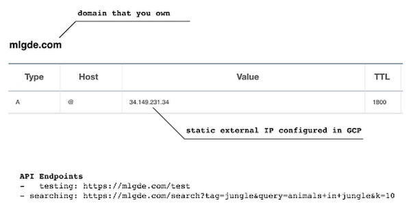
In case you’re wondering why we didn’t deploy this application on App Engine, well that is because of the compute needed to execute the CLIP model. App Engine instance won’t fit in that regime. We could have also incorporated compute-heavy capabilities via a VPC Connector. That is a design choice that you and your team would need to consider. In our experiments, we found the GKE deployment to be easier and suitable for our needs.
Infrastructure for the CLIP model
As mentioned earlier, at the core of our application is the CLIP model. It is computationally a bit more expensive than the regular deep learning models. This is why it makes sense to have the hardware infrastructure set up accordingly to execute it. We ran a small benchmark in order to see how a GPU-based environment could be beneficial here.
We ran the CLIP on a Tesla P100-based machine and also on a standard CPU-only machine 1000 times. The code snippet below is the meat of what we executed:
DEVICE = "cuda" if torch.cuda.is_available() else "cpu"start_time = time.time()for _ in range(1000):with torch.no_grad():model = model.to(DEVICE)inputs = processor(text=[semantic_search_phrase],images=all_images, return_tensors="pt", padding=True)inputs = inputs.to(DEVICE)outputs = model(**inputs)end_time = time.time() - start_timeprint(f"Total time: {end_time:.3f} seconds.")
As somewhat expected, with the GPU, the code took 13 minutes to complete execution. With no GPU, it took about 157 minutes.
It is uncommon to leverage GPUs for model prediction because of cost restrictions, but sometimes we have to access GPUs for deploying a big model like CLIP. We configured a GPU-based cluster on GKE and compared the performance differences with and without it. It took about 1 second to handle a request with GPU and MemoryStore cache while it took more than 4 seconds with MemoryStore only (without the GPUs).
For the purposes of this post, we used a CPU-based cluster on Kubernetes. But It is easy to configure GPU usage in a GKE cluster. This document shows you how to do so. For a short summary, there are two steps. First, a node should be configured with GPUs when creating a GKE cluster. Second, GPU drivers should be installed in GKE nodes. You don’t need to visit and manually install GPU drivers for each node by yourself. Rather you can simply apply the DaemonSet resource to GKE as described here.
Setting up MemoryStore
In this project, we first query the general concept of images to Pixabay, then we filter the images with a semantic query using CLIP. It means we can cache the initially retrieved images from Pixabay for the next specific semantic query. For instance, you may want to search with “gentleman wearing tie” at first, then you may want to retry searching for “gentleman wearing glass”. In this case, the base images remain all the same, so they could be stored in a cache server like Redis.
MemoryStore is a GCP service wrapping the Redis which is an in-memory data store, so you can simply use a standard Redis Python package for accessing it. The only thing to be careful about when provisioning a MemoryStore Redis instance is to make sure it is in the same region where your GKE cluster or Compute Engine instance is.
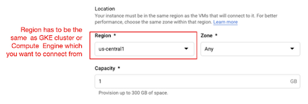
The code snippet below shows how to make a connection to the Redis instance in Python. Nothing specific to GCP, but you only need to be aware of the usage of the standard redis-py package.
# REDISHOST is the IP address to the MemoryStore instanceredis_host = os.environ.get("REDISHOST", "localhost")redis_port = int(os.environ.get("REDISPORT", 6379))redis_client = redis.StrictRedis(host=redis_host, port=redis_port)
After creating a connection, you can store and retrieve data from MemoryStore. There are more advanced use cases of Redis, but we only used exists, get, and set methods for the demonstration purpose. These methods should be very familiar if you know maps, dictionaries, or other similar data structures. For the code portion that uses Redis-related utilities, please refer to the Searcher Python class we discussed in an earlier section.
In the URLs below, you can find side-by-side comparisons of using MemoryStore:
- Without MemoryStore: https://youtu.be/7B88Eyrd-4s
- With MemoryStore (1st try): https://youtu.be/LE6xeEIRuMM
- With MemoryStore (2nd try): https://youtu.be/rRfK17sdk84
Putting everything together
All that’s left now is to collate the different components we developed in the sections above and deploy our application with a frontend. All the frontend-related code is present here.
- The front-end application is written in the Flutter development kit. The main screen contains two text fields for queries to Pixabay and CLIP model respectively. When you click the “Send Query” button, it will send out a RestAPI request to the server. After receiving the result back from the server, the retrieved images from the semantic query will be displayed at the bottom section of the screen.
- Please note that a Flutter application can be deployed to various environments including desktop, web, iOS, and Android. In order to keep as simple as possible, we chose to deploy the application to the GitHub Pages. Whenever there is any change to a client-side source directory, the GitHub Action will be triggered to build a web page and deploy the latest version to the GitHub Pages.
Our final application is deployed here and it looks like so:
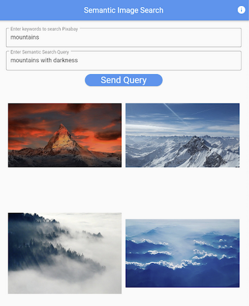
Note that due to constraints, the above-mentioned URL will only be live for one or two months.
It is also possible to redeploy the back-end application with a GitHub Action.
- The very first step is to craft a Dockerfile like below. Since Python is a scripting language, and there are lots of heavy packages that the application is dependent on, it is important to cache the steps. For instance, installing the dependencies should be separated from other commands.
FROM pytorch/pytorch:latestWORKDIR /app# install the dependenciesCOPY requirements.txt requirements.txtRUN pip install -r requirements.txtCOPY . .# set up environment variablesENV PIXABAY_API_KEY="..."ENV REDIS_IN_USE="true"ENV REDISHOST="..."# expose port that Flask app is listening onEXPOSE 8080# run the Flask appCMD [ "python3", "main.py" ]
- With the Dockerfile defined, we can use a GitHub Action like this for automatic deployment.
Edge cases
Since the CLIP model is pre-trained on a large corpus of image and text pairs it’s likely that it may not generalize well to every natural language query we throw at it. Also, because we are limiting the number of images on which the CLIP model can operate, this somehow restricts the expressivity of the model.
We may be able to improve the performance for the second situation by increasing the number of images to be pre-fetched and by indexing them into a low-cost and high-performance database like Datastore.
Costs
In this section, we wanted to provide the readers a breakdown of the costs they might incur in order to consume the various services used throughout the application.
- Frontend hosting
- The front-end application is hosted on GitHub Pages, so there is no expenditure for this.
- Compute Engine
- With an e2-standard-2 instance type without GPUs, the cost is around $48.92 per month. In case you want to add a GPU (NVIDIA K80), the cost goes up to $229.95 per month.
- MemoryStore
- The cost for MemoryStore depends on the size. With 1GB of space, the cost is around $35.77 per month, and whenever you add more GBs the cost will be doubled.
- Google Kubernetes Engine
- The monthly cost for a 3 node GKE cluster with n2-standard-2 (vCPUs: 2, RAM: 8GB without GPUs) is about $170.19. If you add one GPU (NVIDIA K80) to the cluster, the cost goes up to $835.48.
While you may think that is a lot cost-wise, it is good to know that Google gives away free $300 credits when you create a new GCP account. It is still not enough for leveraging GPUs, but it is enough to learn and experiment with GKE and MemoryStore usage.
Conclusion
In this post, we walked through the components needed to build a basic image search utility for natural language queries. We discussed how these different components are connected to each other. Our image search API is able to utilize caching and was deployed on a Kubernetes cluster using GKE. These elements are essential when building a similar service to cater to a much bigger workload. We hope this post will serve as a good starting point for that purpose. Below are some references on similar areas of work that you can explore:
- Building a real-time embeddings similarity matching system
- Detecting image similarity using Spark, LSH and TensorFlow
Acknowledgments: We are grateful to the Google Developers Experts program for supporting us with GCP credits. Thanks to Karl Weinmeister and Soonson Kwon of Google for reviewing the initial draft of this post.
6529
Of your peers have already watched this video.
24:00 Minutes
The most insightful time you'll spend today!
Swarovski’s Journey towards Online and Offline Conversion with Predictive Analytics
Luxury brand and leader in crystals and glass production, Swarovski has charmed customers with its exquisite collections for over 125 years. To understand their customers better and map their online behaviors, Swarovski had to overcome prediction hurdles as majority of the purchases are not frequent or habitual. They are mostly impulse buys or have no rational behind the purchase in order for the brand to accurately map customers’ interest and delight them with relevant personalization or website customization strategy.
Swarovski used a machine learning (ML) model to predict the most performing SKUs and list of products based on both online and offline indicators to target buyers. A score was assigned to each product in the list and was personalized at the country level that delivered relevant insights. Swarovski is aiming to expand the product listing page to personalize at customer level. Watch the video to dive deep into Swarovski’s data analytics efforts to answer complex questions, reporting and prediction using both online and offline data.
More Relevant Stories for Your Company

Ensuring Reliability in a DevOps World: Insights from the 2022 State of DevOps Report
When a software change is deployed — after being designed, coded, tested, packaged, and tested some more — a journey comes to an end. At the same time, a new journey begins: your customer’s relationship with your service. It’s here, in the domain of operations, that abstract risks like launch

The Digital Transformation Journey
Aspiration is easy, but execution is hard. Few concepts illustrate this as well as digital transformations. Most businesses today are at some phase of their digital transformation journey. While some are evaluating strategies and solutions, many companies have already embarked on full-scale project implementations. However, one thing is clear. While

Your Guide to Kubernetes Best Practices
Kubernetes made a splash when it brought containerized app management to the world a few years back. Now, many of us are using it in production to deploy and manage apps at scale. Along the way, we’ve gathered tips and best practices on using Kubernetes and Google Kubernetes Engine (GKE) to your

Swiggy: Delivering Local Food Within 40 Minutes
Founded in 2014, Swiggy started small, delivering food to a few neighborhoods in Bengaluru, India. As the company grew, the team wanted a mapping technology that could help expand the service throughout India. Swiggy needed a scalable mapping platform that covered a wide geographic area and offered tools to help
