





Bit Capital Rolls Out a Digital Financial Solution in Under 3 Months and at 2/3 the Cost

5686
Of your peers have already read this article.
4:00 Minutes
The most insightful time you'll spend today!
In the past few years, a series of new technologies and regulatory changes has been transforming Brazil’s financial industry. The concept of blockchain added security and agility to financial transactions. The open banking system being deployed by the country’s Central Bank (BC) allows for platform integration and data sharing -with the user’s consent- between financial institutions. Recently, the launch of Pix, also by the BC, has shaken the market by creating a new payment method that is instant, free for individuals and 24/7.
Since 2018, the startup Bit Capital has been working on the development of 100%-digital financial solutions in the cloud to help its clients adapt to this new scenario in a convenient way, without the need to build an infrastructure for that or hiring different providers. Pix was not the exception.
In less than 3 months, the team was able to build and go live with a solution that can be used by both direct participants (i.e. those with banking licenses granted by BC) and indirect participants (i.e. companies depending on direct participants to offer payments on Pix) through Bit Capital’s platform.
Besides this differential, Pix and the startup’s other solutions are based on blockchain and Google Cloud’s cloud, ensuring greater security, scalability and availability for customers and allowing for an easy integration between Bit Capital’s platform’s solutions and those from other companies.
“Now we have a platform with an API and various microsservices, allowing clients to connect and develop their own financial product without having to start from scratch.”
—Francesco Miolo, CFO, Bit Capital
A robust structure to handle Pix’s high demand
Bit Capital was established with a certain urgency to develop its platform. The idea was well-developed and customers were interested. The fast deployment of Google Cloud’s tools was one of the main factors that attracted the company to use it as a basis for its infrastructure.
“We managed to deliver everything we have today in Google Cloud with a small team. That was another challenge: being able to grow with a few people,” says Juliano Souza, the startup’s head of IT infrastructure. “We sought other cloud partners, but they had a steep curve. We chose Google Cloud because we needed quick, quality scaling.”
The same thing happened when they built the solution for Pix, despite the specific challenges involved. The BC had performance requirements that led the company to spend some time experimenting until they reached the best suite of tools to meet those requirements. The startup wanted to create a unique architecture that could help both large and small customers and be integrated to the platform’s other microservices.
With the support from Google Cloud’s team to answer doubts and make the best decisions, the solution was built in a few months, at a cost about two-thirds lower than other providers.
The solution’s architecture is based on apps running in Docker in Google Kubernetes Engine (GKE), with interconnected microservices. The blockchain system runs on Compute Engine, its rows are managed in Pub/Sub and Dataflow, and persistent data, in Cloud SQL. Cloud Interconnect is used for the connection with BC. Cloud KMS and Secrets Management store the company’s pre-credentials. All of this is supported by Cloud Load Balancing for load balancing and autoscaling.
According to the team, GKE was essential for the solution’s success. Using infrastructure as code in the tool made uploading of a group of microservices significantly easier. Developers are able to help set up this environment, which has helped spread the DevOps culture in the team. Besides orchestrating and integrating apps, GKE also provides an elastic structure to handle demand peaks and visibility to monitor internal components.
“Google Kubernetes Engine was the only way to ensure availability, observability and elasticity for all clients, whether small, middle-sized or large.”
—Juliano Souza, Head of IT Infrastructure, Bit Capital
Nowadays, the solution’s environment has 20 clusters with over 1,500 pods – 250GB in data per month, providing a robust structure to support a service involving periods of intense demand such as Black Friday.
Ease to monitor, fix and improve
Just 10 days after Pix’s official launch date, the company had its first test: Black Friday. This allowed a major e-commerce customer to test the scale and see the success of the architecture that had been built. “It worked great regarding what the cloud could deliver. And we found what we needed to fix very quickly. Operations [formerly Stackdriver], in particular Cloud Trace, showed us clearly what needed to be done to improve performance,” Souza explains.
Using Operations added reliability by putting deliveries into production. Checking Cloud Trace to see if there were any performance issues and the exact point where they were happening became routine for Bit Capital’s developers. Google Cloud’s security tools and Google Safety Center provided the resources needed to monitor and secure the environment, with automatic data encryption at rest and in transit.
“Google Cloud has security as a premise. When we upload any kind of component, like a database or a virtual machine, the drive is encrypted by default. With other providers, you must specify that you want it encrypted.
”—Juliano Souza, Head of IT Infrastructure, Bit Capital
The easy service monitoring and management accelerates product and technology development because the team no longer needs to worry about infrastructure. Automated management allows professionals to spend more time on new projects and the company’s business. Also, the deployment of services in a Google Cloud multi-region impacts on customer experience, providing high availability for their solutions.
In the coming months, Bit Capital aims to ramp up service usage and the creation of new projects in Google Cloud by adding more customers to Pix’s solution and Banking as a Service (BaaS) solutions. Anthos will be incorporated to the tool suite to make it easier to connect apps with the customers’ on-prem environments. And the deployment of open banking has the potential to be a business driver for the company.
“We joke that we’re already doing open banking, because we have various connections with different providers, which allows us to offer an integrated solution,” says Francesco Miolo, the startup’s CFO. “With the arrival of the new regulations, something we are waiting for since we started out, we will be able, through our platform, to take our customers to the open finance ecosystem, enabling the development of disruptive business models.”
The Query Execution Graph: Your Key to Better BigQuery Analytics

3091
Of your peers have already read this article.
2:30 Minutes
The most insightful time you'll spend today!
BigQuery offers strong query performance, but it is also a complex distributed system with many internal and external factors that can affect query speed. When your queries are running slower than expected or are slower than prior runs, understanding what happened can be a challenge.
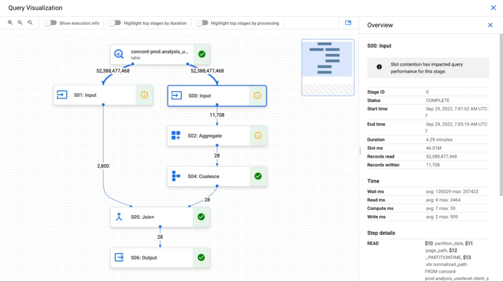
The query execution graph provides an intuitive interface for inspecting query execution details. By using it, you can review the query plan information in graphical format for any query, whether running or completed.
You can also use the query execution graph to get performance insights for queries. Performance insights provide best-effort suggestions to help you improve query performance. Since query performance is multi-faceted, performance insights might only provide a partial picture of the overall query performance.
Execution graph
When BigQuery executes a query job, it converts the declarative SQL statement into a graph of execution, broken up into a series of query stages, which themselves are composed of more granular sets of execution steps. The query execution graph provides a visual representation of the execution stages and shows the corresponding metrics. Not all stages are made equal. Some are more expensive and time consuming than others. The execution graph provides toggles for highlighting critical stages, which makes it easier to spot the potential performance bottlenecks in the query.
Query performance insights
In addition to the detailed execution graph BigQuery also provides specific insights on possible factors that might be slowing query performance.
Slot contention
When you run a query, BigQuery attempts to break up the work needed by your query into tasks. A task is a single slice of data that is input into and output from a stage. A single slot picks up a task and executes that slice of data for the stage. Ideally, BigQuery slots execute tasks in parallel to achieve high performance. Slot contention occurs when your query has many tasks ready for slots to start executing, but BigQuery can’t get enough available slots to execute them.
Insufficient shuffle quota
Before running your query, BigQuery breaks up your query’s logic into stages. BigQuery slots execute the tasks for each stage. When a slot completes the execution of a stage’s tasks, it stores the intermediate results in shuffle. Subsequent stages in your query read data from shuffle to continue your query’s execution. Insufficient shuffle quota occurs when you have more data that needs to get written to shuffle than you have shuffle capacity.
Data input scale change
Getting this performance insight indicates that your query is reading at least 50% more data for a given input table than the last time you ran the query and hence experiencing query slowness. You can use table change history to see if the size of any of the tables used in the query has recently increased.
What’s next?
We continue to work on improving the visualization of the graph. We are working on adding additional metrics to each step and adding more performance insights that will make query diagnosis significantly easier. We are just getting started.
4361
Of your peers have already watched this video.
7:00 Minutes
The most insightful time you'll spend today!
Baking Gets Sweeter: Build ML Models that Help Predict the Best Recipe!
Baking recipes and ML models have one thing in common—they follow a pattern. Machine Learning is all about finding pattern in data sets, you can predict what you are baking based on the core ingredients and their respective amounts! Bread, cake or cookies, watch the video to make you make your baking experiences and learning with ML sweeter.
AutoML Tables, a no-code Google Cloud tool for ML models analyzes data from the databases and spreadsheets to help creates an automatic stats and dashboard with lists of ingredients and their values to predict a new recipe. Watch more episodes from Making with Machine Learning.
New Capabilities in BigQuery to Ease Anomalies Detection in the Absence of Labeled Data

6338
Of your peers have already read this article.
4:00 Minutes
The most insightful time you'll spend today!
When it comes to anomaly detection, one of the key challenges that many organizations face is that it can be difficult to know how to define what an anomaly is. How do you define and anticipate unusual network intrusions, manufacturing defects, or insurance fraud? If you have labeled data with known anomalies, then you can choose from a variety of supervised machine learning model types that are already supported in BigQuery ML. But what can you do if you don’t know what kind of anomaly to expect, and you don’t have labeled data? Unlike typical predictive techniques that leverage supervised learning, organizations may need to be able to detect anomalies in the absence of labeled data.
Today we are announcing the public preview of new anomaly detection capabilities in BigQuery ML that leverage unsupervised machine learning to help you detect anomalies without needing labeled data. Depending on whether or not the training data is time series, users can now detect anomalies in training data or on new input data using a new ML.DETECT_ANOMALIES function (documentation), with the following models:
- Autoencoder model, now in Public Preview (documentation)
- K-means model, already GA (documentation)
- ARIMA_PLUS time series model, already GA (documentation)
How does anomaly detection with ML.DETECT_ANOMALIES work?
To detect anomalies in non-time-series data, you can use:
- K-means clustering models: When you use
ML.DETECT_ANOMALIESwith a k-means model, anomalies are identified based on the value of each input data point’s normalized distance to its nearest cluster. If that distance exceeds a threshold determined by the contamination value provided by the user, the data point is identified as an anomaly. - Autoencoder models: When you use
ML.DETECT_ANOMALIESwith an autoencoder model, anomalies are identified based on the reconstruction error for each data point. If the error exceeds a threshold determined by the contamination value, it is identified as an anomaly.
To detect anomalies in time-series data, you can use:
- ARIMA_PLUS time series models: When you use
ML.DETECT_ANOMALIESwith an ARIMA_PLUS model, anomalies are identified based on the confidence interval for that timestamp. If the probability that the data point at that timestamp occurs outside of the prediction interval exceeds a probability threshold provided by the user, the datapoint is identified as an anomaly.
Below we show code examples of anomaly detection in BigQuery ML for each of the above scenarios.
Anomaly detection with a k-means clustering model
You can now detect anomalies using k-means clustering models, by running ML.DETECT_ANOMALIES to detect anomalies in the training data or in new input data. Begin by creating a k-means clustering model:
Language: SQL
CREATE MODEL `mydataset.my_kmeans_model`OPTIONS(MODEL_TYPE = 'kmeans',NUM_CLUSTERS = 8,KMEANS_INIT_METHOD = 'kmeans++') ASSELECT* EXCEPT(Time, Class)FROM`bigquery-public-data.ml_datasets.ulb_fraud_detection`;
With the k-means clustering model trained, you can now run ML.DETECT_ANOMALIES to detect anomalies in the training data or in new input data.
To detect anomalies in the training data, use ML.DETECT_ANOMALIES with the same data used during training:
Language: SQL
SELECT*FROMML.DETECT_ANOMALIES(MODEL `mydataset.my_kmeans_model`,STRUCT(0.02 AS contamination),TABLE `bigquery-public-data.ml_datasets.ulb_fraud_detection`);
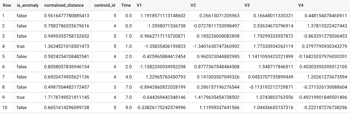
To detect anomalies in new data, use ML.DETECT_ANOMALIES and provide new data as input:
Language: SQL
SELECT*FROMML.DETECT_ANOMALIES(MODEL `mydataset.my_kmeans_model`,STRUCT(0.02 AS contamination),(SELECT * FROM `mydataset.newdata`));

How does anomaly detection work for k-means clustering models?
Anomalies are identified based on the value of each input data point’s normalized distance to its nearest cluster, which, if exceeds a threshold determined by the contamination value, is identified as an anomaly. How does this work exactly? With a k-means model and data as inputs, ML.DETECT_ANOMALIES first computes the absolute distance for each input data point to all cluster centroids in the model, then normalizes each distance by the respective cluster radius (which is defined as the standard deviation of the absolute distances of all points in this cluster to the centroid). For each data point, ML.DETECT_ANOMALIES returns the nearest centroid_id based on normalized_distance, as seen in the screenshot above. The contamination value, specified by the user, determines the threshold of whether a data point is considered an anomaly. For example, a contamination value of 0.1 means that the top 10% of descending normalized distance from the training data will be used as the cut-off threshold. If the normalized distance for a datapoint exceeds the threshold, then it is identified as an anomaly. Setting an appropriate contamination will be highly dependent on the requirements of the user or business.
For more information on anomaly detection with k-means clustering, please see the documentation here.
Anomaly detection with an autoencoder model
You can now detect anomalies using autoencoder models, by running ML.DETECT_ANOMALIES to detect anomalies in the training data or in new input data.
Begin by creating an autoencoder model:
Language: SQL
CREATE MODEL `mydataset.my_autoencoder_model`OPTIONS(model_type='autoencoder',activation_fn='relu',batch_size=8,dropout=0.2,hidden_units=[32, 16, 4, 16, 32],learn_rate=0.001,l1_reg_activation=0.0001,max_iterations=10,optimizer='adam') ASSELECT* EXCEPT(Time, Class)FROM`bigquery-public-data.ml_datasets.ulb_fraud_detection`;
To detect anomalies in the training data, use ML.DETECT_ANOMALIES with the same data used during training:
Language: SQL
SELECT*FROMML.DETECT_ANOMALIES(MODEL `mydataset.my_autoencoder_model`,STRUCT(0.02 AS contamination),TABLE `bigquery-public-data.ml_datasets.ulb_fraud_detection`);
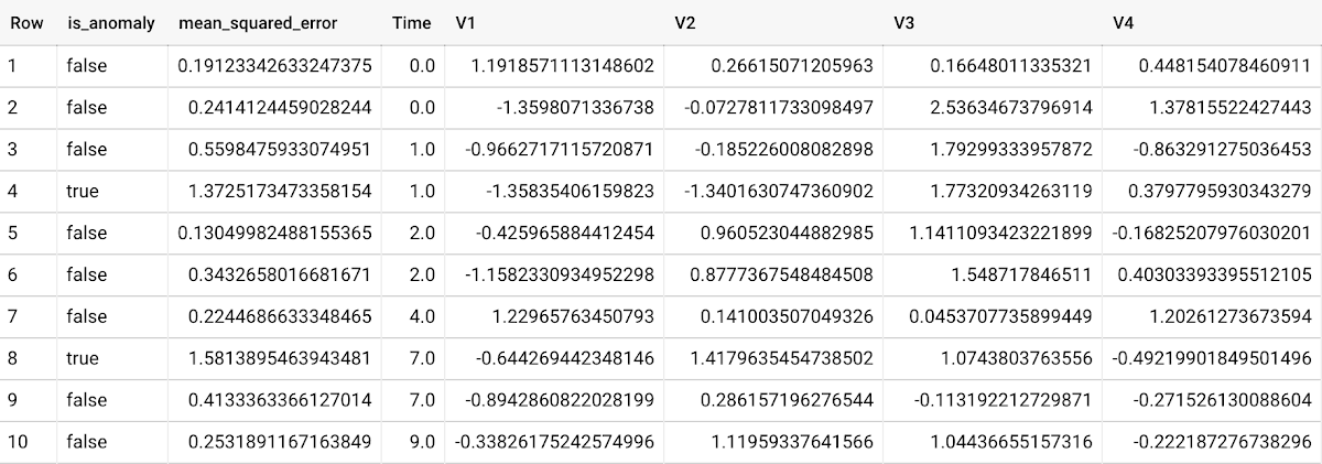
To detect anomalies in new data, use ML.DETECT_ANOMALIES and provide new data as input:
Language: SQL
SELECT*FROMML.DETECT_ANOMALIES(MODEL `mydataset.my_autoencoder_model`,STRUCT(0.02 AS contamination),(SELECT * FROM `mydataset.newdata`));

How does anomaly detection work for autoencoder models?
Anomalies are identified based on the value of each input data point’s reconstructed error, which, if exceeds a threshold determined by the contamination value, is identified as an anomaly. How does this work exactly? With an autoencoder model and data as inputs, ML.DETECT_ANOMALIES first computes the mean_squared_error for each data point between its original values and its reconstructed values. The contamination value, specified by the user, determines the threshold of whether a data point is considered an anomaly. For example, a contamination value of 0.1 means that the top 10% of descending error from the training data will be used as the cut-off threshold. Setting an appropriate contamination will be highly dependent on the requirements of the user or business.
For more information on anomaly detection with autoencoder models, please see the documentation here.
Anomaly detection with an ARIMA_PLUS time-series model
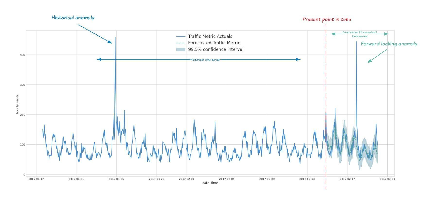
With ML.DETECT_ANOMALIES, you can now detect anomalies using ARIMA_PLUS time series models in the (historical) training data or in new input data. Here are some examples of when might you want to detect anomalies with time-series data:
Detecting anomalies in historical data:
- Cleaning up data for forecasting and modeling purposes, e.g. preprocessing historical time series before using them to train an ML model.
- When you have a large number of retail demand time series (thousands of products across hundreds of stores or zip codes), you may want to quickly identify which stores and product categories had anomalous sales patterns, and then perform a deeper analysis of why that was the case.
Forward looking anomaly detection:
- Detecting consumer behavior and pricing anomalies as early as possible: e.g. if traffic to a specific product page suddenly and unexpectedly spikes, it might be because of an error in the pricing process that leads to an unusually low price.
- When you have a large number of retail demand time series (thousands of products across hundreds of stores or zip codes), you would like to identify which stores and product categories had anomalous sales patterns based on your forecasts, so you can quickly respond to any unexpected spikes or dips.
How do you detect anomalies using ARIMA_PLUS? Begin by creating an ARIMA_PLUS time series model:
Language: SQL
CREATE OR REPLACE MODEL mydataset.my_arima_plus_modelOPTIONS(MODEL_TYPE='ARIMA_PLUS',TIME_SERIES_TIMESTAMP_COL='date',TIME_SERIES_DATA_COL='total_amount_sold',TIME_SERIES_ID_COL='item_name',HOLIDAY_REGION='US') ASSELECTdate,item_description AS item_name,SUM(bottles_sold) AS total_amount_soldFROM`bigquery-public-data.iowa_liquor_sales.sales`GROUP BYdate,item_nameHAVINGdate BETWEEN DATE('2016-01-04') AND DATE('2017-06-01')AND item_name IN ("Black Velvet", "Captain Morgan Spiced Rum","Hawkeye Vodka", "Five O'Clock Vodka", "Fireball Cinnamon Whiskey");
To detect anomalies in the training data, use ML.DETECT_ANOMALIES with the model obtained above:
Language: SQL
SELECT*FROMML.DETECT_ANOMALIES(MODEL `mydataset.my_arima_plus_model`,STRUCT(0.8 AS anomaly_prob_threshold));
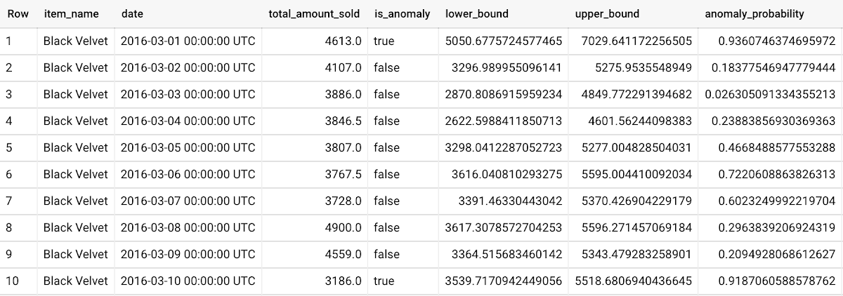
To detect anomalies in new data, use ML.DETECT_ANOMALIES and provide new data as input:
Language: SQL
WITHnew_data AS (SELECTdate,item_description AS item_name,SUM(bottles_sold) AS total_amount_soldFROM`bigquery-public-data.iowa_liquor_sales.sales`GROUP BYdate,item_nameHAVINGdate BETWEEN DATE('2017-06-02')AND DATE('2017-10-01')AND item_name IN ('Black Velvet','Captain Morgan Spiced Rum','Hawkeye Vodka',"Five O'Clock Vodka",'Fireball Cinnamon Whiskey') )SELECT*FROMML.DETECT_ANOMALIES(MODEL `mydataset.my_arima_plus_model`,STRUCT(0.8 AS anomaly_prob_threshold),(SELECT*FROMnew_data));
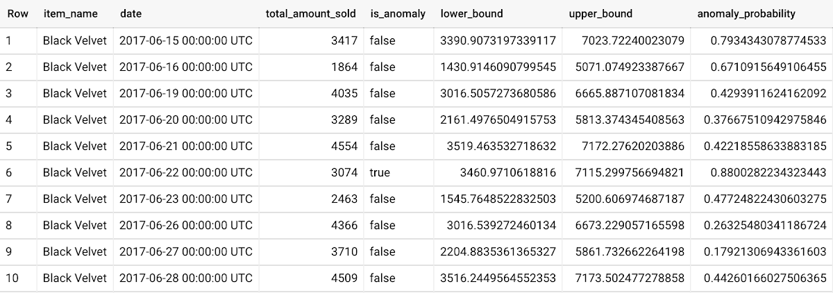
For more information on anomaly detection with ARIMA_PLUS time series models, please see the documentation here.
Thanks to the BigQuery ML team, especially Abhinav Khushraj, Abhishek Kashyap, Amir Hormati, Jerry Ye, Xi Cheng, Skander Hannachi, Steve Walker, and Stephanie Wang.
S4 Agtech Transforms Agriculture with Google Cloud

7494
Of your peers have already read this article.
8:30 Minutes
The most insightful time you'll spend today!
Like countless other industries, farming is going digital and undergoing big changes—driven by access to more actionable information. The agriculture business can now gather and analyze georeferenced data from satellites, combined with data from IoT sensors in fields, crop rotation and yield histories, weather patterns, seed genotypes and soil composition to help increase the quantity and quality of crops.
This is essential for businesses in the agriculture industry, but it’s also critical to address growing food shortages around the world.
At S4, we create technology to de-risk crop production. We provide customers seeking agricultural risk management solutions with the tools to make better, data-driven decisions for their crop planning, based on machine learning and proprietary algorithms.
We interpret plant evolution on a global scale with predictive modeling and analytics, and offer super-efficient risk-transferring solutions. Our multi-cloud platform includes a petabyte-scale database, an open source stack, and—after 50 proof-of-concept evaluations—BigQuery for our data warehouse and the Cloud SQL database service to handle OLTP queries to our PostgreSQL database.
These PoCs included, among others, Microsoft Azure Data Lake Analytics, IBM Netezza, Postgres/PostGIS running on IBM bare-metal servers with SATA SSDs and on Google’s Compute Engine with NVMe disks, and on-premises memSQL, CitusData and Yandex ClickHouse.
Weeding out risk in an uncertain market
According to recent research, climate extreme events like drought, heat waves, and heavy precipitation are responsible for 18-43% of global variation in crop yields for maize, spring wheat, rice, and soybeans. This is a clear trend for other crops as well. Such variation poses risks of food shortages as well as large financial risks to farmers, insurers, and regions dependent on successful crop yields. Also, it creates vast humanitarian difficulties.
Our mission at S4 is to help de-risk crop production by matching the right data with analytics tools so farmers and other participants in the agricultural value chain can plan better, resulting in more reliable food supplies.
In a nutshell, we create indices out of biological assets. These indices measure yield losses on crops that are caused by the effects of weather and other factors, which are then used as underlying assets for products, such as swap/derivative contracts and parametric insurance policies, to transfer risk to the financial markets.
We enable insurers and lenders to buy and sell agricultural risks through the futures market. Also, our other products help farmers and seed and fertilizer companies provide customized genotype recommendations and fertilization requirements. This helps to optimize planting by geography, resources, and crop species, monitor phenological, pests and humidity evolution throughout the crop season, and estimate yields.
Local communities benefit from S4’s technology, as the ability to manage weather risks allows farmers to stabilize their cash flows, invest more to produce more with fewer risks, and develop in a more sustainable manner.
Growing data sources, reducing costs, accelerating performance
With the volume of diverse data sources and analytical complexity both growing at a very fast pace, we decided that using a major cloud services provider with a broad roadmap and global partnerships would be beneficial to S4’s future evolution.
At the same time, we wanted to bring our services to users faster and cut costs by consolidating our on-premises technology stack. When we started evaluating providers, our leading criteria included a powerful geospatial database and data analytics tools along with excellent support, all at a competitive price. GCP prevailed in nearly all criteria categories among the 50 companies we measured.
Our previous platform architecture included a hybrid relational database that used Compute Engine for virtual machines and Cloud Storage for database backup. The RDBMS was slow. Maintaining our own data warehouse was complex and expensive.
We wanted to use machine learning and neural networks, but couldn’t do so easily and affordably. The complexity of that system meant that products or services requiring small changes or additions to the data model translated to expensive expansions of infrastructure or project time.
Also, agronomical or product teams couldn’t test these changes by themselves, always requiring the intervention on no small part of the IT team, which led to further delays.
We added GCP services like BigQuery as S4’s cloud data warehouse and use BigQuery GIS for geospatial analysis, Cloud Dataflow for simplified stream and batch data processing, and Cloud SQL for queries to the S4 database platform, which have all made a huge impact on our services and bottom line.
Database and analytics costs have decreased by 40% and customers are receiving our analytical results 25% faster. In addition, we’ve eliminated the time-consuming downloading of images, reducing storage and processing costs by 80%, because we no longer need expensive tools licenses, and have greatly reduced classification processing times.
Our customers working in the agriculture industry are also benefiting from this infrastructure change. They are now able to speed up their data analytics using our GCP-based platform.
“S4 products and technologies unlock the full potential of satellite imagery for crop prescriptions, monitoring and yield estimates,” says Nicolás Loria, Manager of Marketing Services, Southern Cone, Corteva Agriscience.
“We’ve worked with S4 for the last three (and starting year number four) crop seasons as its team capabilities, data integration capacities, and analytics insights have allowed Corteva to perform an entire new solution. Thanks to S4’s customized 360° approach, fast response and delivery times, we have safely outsourced our remote crop analytic technical needs.”
Also, this new architecture has allowed us to scale our models and databases with almost no limits, at a fraction of the cost vs. the previous models.
We’ve saved a lot of time on executing processes and reduced work needed by our internal teams to do certain tasks, like preparing images, converting them, validating results, and more. Using Google Earth Engine has decreased the execution time of daily tasks anywhere from 50% to 90% of the previous time, going from an average time of 30 minutes to between four and 15 minutes, depending on the task.
In addition to saving money and time, we are able to focus on innovation with the GCP performance and features we’re using. We’re able to seamlessly add satellite data to analytics using both public datasets and our own private data, and deliver GIS data management, analytics, crop classification and monitoring in real time.
We can do semi-automatic crop classification and classification using spectral signatures with Google Earth Engine. Later this year, we’ll be using neural networks for pattern recognition and machine learning in new applications to improve crop yields and fine-tune risk models. And using GCP and Google Earth Engine infrastructure means we can run models for customers in South America and around the world, since Google Earth Engine has global satellite imagery available.
We’ve heard from our customer Indigo Argentina that they’re able to bring customers data insights faster.
“We are working with S4 in the development of two different applications for satellite crop monitoring and yield assessment,” says Carlos Becco, CEO, Indigo Argentina. “S4’s technology allowed us to manage and analyze multiple sources and layers of information in real time, letting us uncover valuable insights in Indigo’s own microbiome technologies, and at a very competitive cost.”
Analytical products and app development thrive with GCP
With GCP, we are updating and improving algorithms that we built manually with machine learning processes to develop drought indices for upcoming crop seasons. Algorithms can recognize specific phases of crop phenology (e.g., bud burst, flowering, fruiting, leaf fall) and correlate them with photosynthetic activity, light, water, temperature, radiation, and plant genetics factors. Other analytical products like crop monitoring, pre-planting recommendations, financial scoring, and yield estimation can now do a lot more for users by offering multiple layers and datasets, faster image processing, and real-time access via APIs.
We also replaced our bare-metal S4 app deployment with the App Engine serverless application platform. It provides tighter integration between the S4 platform and our BigQuery data warehouse for integration with marketplaces and third-party solutions.
We get all of these Google Cloud features with all the benefits of managed cloud services, from multiversioning and security to automatic backups and high availability.
At S4, we trust technology to decode plant growth and help protect farmers and their communities from climate change. With growing food shortages due to increasing populations and intensifying weather, data and analytics can have a huge impact in lowering financial risks and improving agricultural yields. It’s one sector where cloud, database, analytics, and other technologies are combining to improve business outcomes and affect the lives of billions of people. Learn more about S4’s work and learn more about data analytics on Google Cloud.
Geospatial Data for Business Apps Drive Sustainable and Accurate Decision-making

4360
Of your peers have already read this article.
1:30 Minutes
The most insightful time you'll spend today!
Organizations that collect geospatial data can use that information to understand their operations, help make better business decisions, and power innovation. Traditionally, organizations have required deep GIS expertise and tooling in order to deliver geospatial insights. In this post, we outline some ways that geospatial data can be used in various business applications.
Assessing environmental risk
Governments and businesses involved in insurance underwriting, property management, agriculture technology, and related areas are increasingly concerned with risks posed by environmental conditions. Historical models that predict natural disasters like pollution, flooding, and wildfires are becoming less accurate as real-world conditions change. Therefore, organizations are incorporating real-time and historical data into a geospatial analytics platform and using predictive modeling to more effectively plan for risk and to forecast weather.
Selecting sites and planning expansion
Businesses that have storefronts, such as retailers and restaurants, can find the best locations for their stores by using geospatial data like population density to simulate new locations and to predict financial outcomes. Telecom providers can use geospatial data in a similar way to determine the optimal locations for cell towers. A site selection solution can combine proprietary site metrics with publicly-available data like traffic patterns and geographic mobility to help organizations make better decisions about site selection, site rationalization, and expansion strategy.
Planning logistics and transport
For freight companies, courier services, ride-hailing services, and other companies that manage fleets, it’s critical to incorporate geospatial context into business decision-making. Fleet management operations include optimizing last-mile logistics, analyzing telematics data from vehicles for self-driving cars, managing precision railroading, and improving mobility planning. Managing all of these operations relies extensively on geospatial context. Organizations can create a digital twin of their supply chain that includes geospatial data to mitigate supply chain risk, design for sustainability, and minimize their carbon footprint.
Understanding and improving soil health and yield
AgTech companies and other organizations that practice precision agriculture can use a scalable analytics platform to analyze millions of acres of land. These insights help organizations understand soil characteristics and help them analyze the interactions among variables that affect crop production. Companies can load topography data, climate data, soil biomass data, and other contextual data from public data sources. They can then combine this information with data about local conditions to make better planting and land-management decisions. Mapping this information using geospatial analytics not only lets organizations actively monitor crop health and manage crops, but it can help farmers determine the most suitable land for a given crop and to assess risk from weather conditions.
Managing sustainable development
Geospatial data can help organizations map economic, environmental, and social conditions to better understand the geographies in which they conduct business. By taking into account environmental and socio-economic phenomena like poverty, pollution, and vulnerable populations, organizations can determine focus areas for protecting and preserving the environment, such as reducing deforestation and soil erosion. Similarly, geospatial data can help organizations design data-driven health and safety interventions. Geospatial analytics can also help an organization meet its commitments to sustainability standards through sustainable and ethical sourcing. Using geospatial analytics, organizations can track, monitor, and optimize the end-to-end supply chain from the source of raw materials to the destination of the final product.
What’s next
Google Cloud provides a full suite of geospatial analytics and machine learning capabilities that can help you make more accurate and sustainable business decisions without the complexity and expense of managing traditional GIS infrastructure. Get started today by learning how you can use Google Cloud features to get insights from your geospatial data, see Geospatial analytics architecture.
Acknowledgements: We’d like to thank Chad Jennings, Lak Lakshmanan, Kannappan Sirchabesan, Mike Pope, and Michael Hao for their contributions to this blog post and the Geospatial Analytics architecture.
More Relevant Stories for Your Company

How Major League Baseball Migrated from Teradata to BigQuery
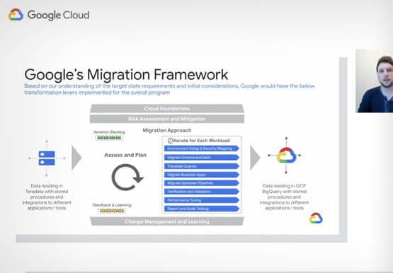
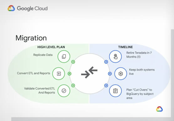
Ever wondered how to jumpstart a migration from your legacy on-premises or cloud data warehouse to BigQuery? In this video Robert Goretsky, VP, Data Engineering, Major League Baseball and Ryan McDowell, Cloud Data Engineer, Google Cloud show you how. They offer a deep-dive into MLB’s Teradata to BigQuery migration journey.

Report on API-led Digital Transformations in 2020 and the Future
In 2020, many businesses across industries turned their focus and investments towards digital strategies. APIs being an integral part of every organization's digital disruption, will grow in relevance throughout 2021. Read the report to gain more insights on driving API-led digital transformations and in-depth analysis of Google Cloud's Apigee API

How AI is Revolutionizing Retail: Lessons for Marketers
Reach the Right Customers How can AI help you target customers who are looking for products like yours? The challenge: This customer wants to buy the best cat food for her pets. How AI Works The Result A targeted offer for a discount on luxury cat food is shown to


Video: How AI is Helping Biologists Protect Wildlife
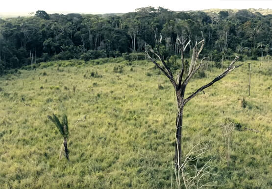
According to the World Wildlife Fund, vertebrate populations have shrunk an average of 60 percent since the 1970s. And a recent UN global assessment found that we’re at risk of losing one million species to extinction, many of which may become extinct within the next decade. To better protect wildlife, seven organizations, led
