





Autoclass: Simplify and Automate Cost Optimization for Cloud Storage

3231
Of your peers have already read this article.
3:00 Minutes
The most insightful time you'll spend today!
There is a data explosion challenge that most IT admins and companies are tackling regularly. The cost-effectiveness, durability and scalability make object storage the first choice for unstructured data. Cloud Storage is an object storage service capable of storing data at exabyte scale and easily managing billions, if not trillions, of objects. However, cost optimization for data stored in object storage is a hard problem.
Choosing the right storage class for your data requires you to know about the access patterns for this data. However, if the access patterns are unknown or unpredictable, it’s often difficult for customers to choose the right storage class for their data. Data placement can have a significant impact on cost as the storage price for the archive class is 6% the storage price for the standard storage class. Having frequently accessed data in colder storage classes can lead to unexpected operations charges. Having data that is never accessed in standard storage can lead to large at-rest storage bills.
As IT administrators and organizations enable different applications and workloads to start leveraging object storage at massive scale, optimizing for cost is only getting exponentially harder to solve. As they migrate workloads to cloud they would like to have predictability and control in their overall storage spend. Wouldn’t it be great if there was a way to automatically place your data in the best storage class?
Introducing Autoclass – a new managed data placement service for Cloud Storage.
Simplifying Lifecycle Management while Reducing TCO
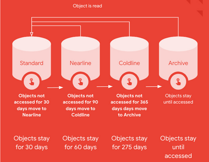
Autoclass is an easy to use bucket-level setting that simplifies and automates lifecycle management of all your Cloud Storage data based on last access time.
This is very useful for workloads with unpredictable and unknown access patterns. It automatically moves data that is not accessed to colder storage classes to reduce at-rest storage cost. When cold data is accessed, it is automatically promoted to Standard storage class to optimize the operations costs for future accesses.
Autoclass automatically delivers cost savings and removes inefficiencies by moving data to the storage class with the most favorable pricing for customer workloads.
It helps organizations achieve price predictability by removing surcharges associated with colder storage classes – there are no early deletion fees, retrieval fees or operations charges for class transitions when Autoclass is enabled on a bucket.
What are customers saying about Autoclass?
“Redivis is a data platform for academic research. We connect data managers with researchers to discover, understand, and analyze Petabytes of data. With Cloud Storage Autoclass, this shifts the paradigm in the research community,” said Ian Matthews, co-founder and CEO of Redivis Inc. “We can now keep more data for longer periods of time while reducing our costs. In fact, I’d estimate 90% of our data will benefit from Autoclass.”
Ian adds “Not only would it cost valuable engineering resources to build cost-optimization ourselves, but it would open us up to potentially costly mistakes in which we incur retrieval charges for prematurely archived data. Autoclass helps us reduce storage costs and achieve price predictability in a simple and automated way.”
Using Autoclass
With this release, Autoclass can be enabled when you create a new Cloud Storage bucket by using CLI, API, or Cloud Console. Once enabled on a bucket, Autoclass will manage the lifecycle of all objects that are uploaded to the bucket until disabled.
If you choose to disable Autoclass, all the objects in the bucket will remain in their current storage class. This disablement doesn’t require any data movement or any changes to storage classes of objects and hence, incurs no charge.
The support for enabling Autoclass on existing Cloud Storage buckets will be available in an upcoming release in 2023.
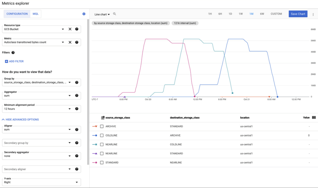
All transitions carried out by Autoclass can be observed using Cloud Monitoring dashboards. This provides easy observability and allows you to validate what Autoclass is doing for your data in an automated way. These dashboards can leverage 2 new Cloud metrics published for Autoclass:
- Number of objects transitioned by Autoclass (autoclass/transition_operation_count)
- Number of bytes transitioned between classes by Autoclass (autoclass/transitioned_bytes_count)
Getting Started
All Cloud Storage customers can enable Autoclass on their new buckets and realize the cost savings for themselves. For more information and detailed instructions on how to enable Autoclass, refer to the documentation here.
Canadian Bank’s SAP Workload Moved to BigQuery Helps Unlock New Business Opportunities

7363
Of your peers have already read this article.
2:00 Minutes
The most insightful time you'll spend today!
When ATB Financial decided to migrate its vast SAP landscape to the cloud, the primary goal was to focus on things that matter to customers as opposed to IT infrastructure. Based in Alberta, Canada, ATB Financial serves over 800,000 customers through hundreds of branches as well as digital banking options. To keep pace with competition from large banks and FinTech startups and to meet the increasing 24/7 demands of customers, digital transformation was a must. To support this new mandate, in 2019, ATB migrated its extensive SAP backbone to Google Cloud. In addition to SAP S/4 HANA, ATB runs SAP financial services, core banking, payment engine, CRM and business warehouse on Google Cloud.
In parallel, changes were needed to ATB’s legacy data platform. The platform had stability and reliability issues and also suffered from a lack of historical data governance. Analytics processes were ad hoc and manual. The legacy data environment was also not set up to tackle future business requirements that come with a high dependency on real-time data analysis and insights.
After evaluating several potential solutions, ATB chose BigQuery as a serverless data warehouse and data lake for its next-generation, cloud-native architecture. “BigQuery is a core component of what we call our data exposure enablement platform, or DEEP,” explains Dan Semmens, Head of Data and AI at ATB Financial. According to Semmens, DEEP consists of four pillars, all of which depend on Google Cloud and BigQuery to be successful:
- Real-time data acquisition: ATB uses BigQuery throughout its data pipeline, starting with sourcing, processing, and preparation, moving along to storage and organization, then discovery and access, and finally consumption and servicing. So far, ATB has ingested and classified 80% of its core SAP banking data as well as data from a number of its third-party partners, such as its treasury and cash management platform provider, its credit card provider, and its call center software.
- Data enrichment: Before migrating to Google Cloud, ATB managed a number of disconnected technologies that made data consolidation difficult. The legacy environment could handle only structured data, whereas Google Cloud and BigQuery lets the bank incorporate unstructured data sets, including sensor data, social network activity, voice, text, and images. ATB’s data enrichment program has enabled more than 160 of the bank’s top-priority insights running on BigQuery, including credit health decision models, financial reporting, and forecasting, as well as operational reporting for departments across the organization. Jobs such as marketing campaigns and month-end processes that used to take five to eight hours now run in seconds, saving over CA$2.24 million in productivity.
- Self-service analytics: Data for self-service reporting, dashboarding, and visualization is now available for ATB’s 400+ business users and data analysts. Previously, bringing data and analytics to the business users who needed it while ensuring security was burdensome for IT, fraught with recurrent data preparation and other highly manual elements. Now, ATB automates much of its data protection and governance controls through the entire data lifecycle management process. Data access is not only open to more team members but it is faster and easier to acquire without compromising security. And it’s not just raw data that users can access. ATB uses BigQuery to define its enterprise data models and create what it calls its data service layer to make it easier for team members to visualize their data.
- AI-assisted analytics and automation: Through Google Cloud and BigQuery, ATB has been able to publish data and ML models that provide alerts and notifications via APIs to customer service agents. These real-time recommendations allow customer service agents to provide more tailored service with contextualized advice and suggested new services. So far, the company has deployed more than 40 ML models to generate over 20,000 AI-assisted conversations per month. Thanks to improved customer advocacy and less churn, the bank has realized more than CA$4 million in operating revenue. During the ongoing COVID crisis, the system was also able to predict when business and personal banking customers were experiencing financial distress so that a relationship manager could proactively reach out to offer support, such as payment deferral or loan restructuring. The AI tools provided by BigQuery are also helping ATB detect fraud that previously evaded rules-based fraud detection by using broader sets of timely and accurate data.
Thanks to the speed and ease of moving data from SAP to BigQuery, ATB is using artificial intelligence (AI) and machine learning (ML) to do things it previously hadn’t thought possible, including sophisticated fraud prevention models, product recommendations, and enriched CRM data that improves the customer experience.
Using the power of Google Cloud and BigQuery, ATB Financial has been able to draw more value from its SAP data while lowering cost and improving security and reliability. Speed to provide data sets and insights to internal team members has improved 30%. The bank also has seen a 15x reduction in performance incidents while improving data governance and security. Dan Semmens projects that the digital transformation strategy built on Google Cloud and BigQuery has both saved millions compared to its on-premises environment and has also realized millions in new business opportunities.
Semmens is looking toward the future that includes initiatives like Open Banking and greater ability to provide real time personalized advice for customers to drive revenue growth. “We see our data platform as foundational to ATB’s 10-year strategy,” he says. “The work we’ve undertaken over the past 18 months has enabled critical functionality for that future.”
Learn more about how ATB Financial is leveraging BigQuery to gain more from SAP data. Visit us here to explore how Google Cloud, BigQuery, and other tools can unlock the full value of your SAP enterprise data.
How AI-powered ML Models Helps Run Unemployment Claims Verification at Scale

8400
Of your peers have already read this article.
2:00 Minutes
The most insightful time you'll spend today!
With unemployment application submissions reaching record numbers over the past year, state and local agencies in the United States have faced the challenge of processing unprecedented numbers of claims per week. The digital infrastructure most agencies have in place is unable to handle this volume, resulting in constituents waiting longer, and bad actors taking advantage of vulnerable systems. The Department of Labor Inspector General estimates that $63 billion in claims distributed is either an improper payment or fraud.
Validating claims also requires secure data sharing with other agencies for document and identity verification. Government leaders need a way to allow case adjudicators to quickly and confidently release backlogged claims, integrate with existing systems, and segment legitimate claims from potentially fraudulent ones — all within limited government budgets — securely and at scale.
Implementing a fraud detection solution on Google Cloud
States were under pressure to release payments, while also filtering out potentially fraudulent claims. SpringML and Google Cloud developed a framework to give adjudicators a reliable verification process that quickly filters potentially fraudulent claims, while processing the remaining claims so benefits reach citizens in a timely manner. SpringML and Google Cloud, applied AI-powered machine learning models to detect anomalous patterns in large datasets. Using Google Cloud tools, SpringML implemented a solution to streamline workflows, improve efficiencies, automate processes and identify potentially fraudulent claims.
SpringML used a variety of Google Cloud products to deliver a fraud detection solution, including:
- Google Cloud Storage to store and manage data
- BigQuery to store tabular data and BigQuery Machine Learning (BQML) to conduct machine learning on that data
- AutoML solutions to build predictive models and risk scoring
- Visualization tools such as Looker and Data Studio to present data and help government leaders make informed decisions.
Implementing machine learning to detect improper payments allows agencies to classify claims as “fraud” or “not fraud” based on the number of flags, as well as prioritize the most urgent claims. Deploying intelligent virtual agents to handle frequently asked questions meant that live agents could focus their time on more challenging cases.
Even once the pandemic is behind us, there will be bad actors trying to take advantage of overwhelmed or legacy systems. We’ve identified a few best practices for agencies managing enormous case loads and looking to improve improper payment analytics:
- Move your systems to the cloud. Many on-premises legacy systems can’t update their applications and scale to meet the volume of claims. Moving to a cloud environment enables rapid solution deployment and ingestion of large amounts of data without fear of overloading the system. The cloud scales with you–cost-effectively and securely.
- Understand patterns in the data. The answer is always in the data — we used deep analysis to help uncover suspicious patterns in large data sets. We implemented unsupervised machine learning to learn behaviors and create configurable rules that adjust to new information that comes into the system. We can uncover patterns that are likely associated with fraud – ones that a human might have missed.
- Use AI/ML tools to automate your existing systems and teams. These tools enable humans to work smarter and more efficiently. We automate anomaly detection and create dashboards for adjudicators to rapidly process claims. We are enabling the Wisconsin Department of Workforce Development by implementing automatic calculations and processing of recharge amounts, resulting in faster processing times and fewer human errors. Proactive fraud detection and timely calculation of recharge payment allowed DWD to ensure the benefits reached the right individuals.
- Build flexibility into your systems. We discovered that fraud patterns change over time. For instance,flags for fraud during March-May 2020 were vastly different from those we found in June-July 2020. Google Cloud tools make it easy to continually update algorithms to detect patterns and integrate external data sources.
Using Google Cloud tools, we can update digital infrastructure and incorporate machine learning best practices to help organizations efficiently process large volumes of claims and identify high probability fraudulent ones. SpringML provides consulting and implementation services and industry-specific analytics solutions that deliver high-impact business value to accelerate data-driven digital transformation. Learn more about fraud detection and how to improve improper payments analytics by watching our webinar.
How to Enhance Incremental Pipeline Performance while Ingesting Data into BigQuery

6332
Of your peers have already read this article.
3:00 Minutes
The most insightful time you'll spend today!
When you build a data warehouse, the important question is how to ingest data from the source system to the data warehouse. If the table is small you can fully reload a table on a regular basis, however, if the table is large a common technique is to perform incremental table updates. This post demonstrates how you can enhance incremental pipeline performance when you ingest data into BigQuery.
Setting up a standard incremental data ingestion pipeline
We will use the below example to illustrate a common ingestion pipeline that incrementally updates a data warehouse table. Let’s say that you ingest data into BigQuery from a large and frequently updated table in the source system, and you have Staging and Reporting areas (datasets) in BigQuery.

The Reporting area in BigQuery stores the most recent, full data that has been ingested from the source system tables. Usually you create the base table as a full snapshot of the source system table. In our running example, we use BigQuery public data as the source system and create reporting.base_table as shown below. In our example each row is identified by a unique key which consists of two columns: block_hash and log_index.
CREATE TABLE reporting.base_table --156 GB processedPARTITION BY TIMESTAMP_TRUNC(block_timestamp, DAY) ASSELECT log_index, data, topics, block_timestamp, block_hashFROM bigquery-public-data.crypto_ethereum.logsWHERE block_timestamp BETWEEN TIMESTAMP '2020-01-01' AND TIMESTAMP '2020-11-30';
In data warehouses it is common to partition a large base table by a datetime column that has a business meaning. For example, it may be a transaction timestamp, or datetime when some business event happened, etc. The idea is that data analysts who use the data warehouse usually need to analyze only some range of dates and rarely need the full data. In our example, we partition the base table by block_timestamp which comes from the source system.
After ingesting the initial snapshot you need to capture changes that happen in the source system table and update the reporting base table accordingly. This is when the Staging area comes into the picture. The staging table will contain captured data changes that you will merge into the base table. Let’s say that in our source system on a regular basis we have a set of new rows and also some updated records. In our example we mock the staging data as follows: first, we create new data, than we mock the updated records:
CREATE TABLE staging.load_delta AS --5 GB processedSELECT log_index, data, topics, block_timestamp, block_hashFROM bigquery-public-data.crypto_ethereum.logsWHERE block_timestamp BETWEEN TIMESTAMP '2020-12-01' AND TIMESTAMP '2020-12-07';INSERT INTO staging.load_delta --2 GB processedSELECT log_index, CONCAT(data, RAND()), topics, block_timestamp, block_hashFROM bigquery-public-data.crypto_ethereum.logs TABLESAMPLE SYSTEM (5 PERCENT)WHERE block_timestamp BETWEEN TIMESTAMP '2020-10-01' AND TIMESTAMP '2020-11-30';
Next, the pipeline merges the staging data into the base table. It joins two tables by unique key and than updates the changed value or inserts a new row
MERGE INTO reporting.base_table T --161 GB processedUSING staging.load_delta SON T.block_hash = S.block_hashAND T.log_index = S.log_indexWHEN MATCHED THEN UPDATE SETT.data = S.dataWHEN NOT MATCHED THEN INSERT (log_index, data, topics, block_timestamp, block_hash)VALUES (log_index, data, topics, block_timestamp, block_hash);
It is often the case that the staging table contains keys from various partitions but the number of those partitions are relatively small. It holds, for instance, because in the source system the recently added data may get changed due to some initial errors or ongoing processes but older records are rarely updated. However, when the above MERGE gets executed, BigQuery scans all partitions in the base table and processes 161 GB of data. You might add additional join condition on block_timestamp:
MERGE INTO reporting.base_table T --161 GB processedUSING staging.load_delta SON T.block_hash = S.block_hashAND T.log_index = S.log_indexAND T.block_timestamp = S.block_timestampWHEN MATCHED THEN UPDATE SETT.data = S.dataWHEN NOT MATCHED THEN INSERT (log_index, data, topics, block_timestamp, block_hash)VALUES (log_index, data, topics, block_timestamp, block_hash);
But BigQuery would still scan all partitions in the base table because condition T.block_timestamp = S.block_timestamp is a dynamic predicate and BigQuery doesn’t automatically push such predicates down from one table to another in MERGE.
Can you improve the MERGE efficiency by making it scan less data? The answer is Yes.
As described in the MERGE documentation, pruning conditions may be located in a subquery filter, a merge_condition filter, or a search_condition filter. In this post we show how you can leverage the first two. The main idea is to turn a dynamic predicate into a static predicate.
Steps to enhance your ingestion pipeline
The initial step is to compute the range of partitions that will be updated during the MERGE and store it in a variable. As was mentioned above, in data ingestion pipelines, staging tables are usually small so the cost of the computation is relatively low.
DECLARE src_range STRUCT<date_min TIMESTAMP, date_max TIMESTAMP> --115 MB processedDEFAULT(SELECT STRUCT(MIN(block_timestamp) AS date_min,MAX(block_timestamp) AS date_max) FROM staging.load_delta);
Based on your existing ETL/ELT pipeline, you can add the above code as-is to your pipeline or you can compute date_min, data_max as part of some already existing transformation step. Alternatively, date_min, data_max can be computed on the Source System side while capturing the next ingestion data batch.
After computing date_min, date_max you pass those values to the MERGE statement as static predicates. There are several ways to enhance the MERGE and prune partitions in the base table based on precomputed date_min, data_max.
If your initial MERGE statement uses a subquery, you can incorporate a new filter into it:
BEGINDECLARE src_range STRUCT<date_min TIMESTAMP, date_max TIMESTAMP> --115 MB processedDEFAULT(SELECT STRUCT(MIN(block_timestamp) AS date_min,MAX(block_timestamp) AS date_max) FROM staging.load_delta);MERGE INTO reporting.base_table T --41 GB processedUSING (SELECT *FROM staging.load_deltaWHERE block_timestamp BETWEEN src_range.date_min AND src_range.date_max) SON T.block_hash = S.block_hashAND T.log_index = S.log_indexAND T.block_timestamp = S.block_timestampWHEN MATCHED THEN UPDATE SETT.data = S.dataWHEN NOT MATCHED THEN INSERT (log_index, data, topics, block_timestamp, block_hash)VALUES (log_index, data, topics, block_timestamp, block_hash);END;
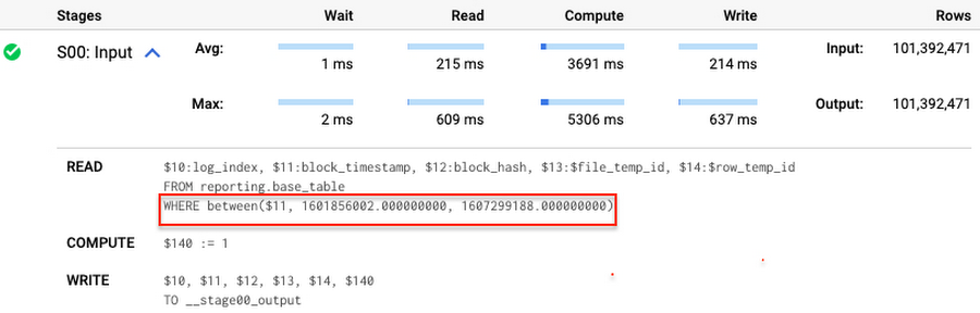
Note that you add the static filter to the staging table and keep T.block_timestamp = S.block_timestamp to convey to BigQuery that it can push that filter to the base table. This MERGE processes 41 GB of data in contrast to the initial 161 GB. You can see in the query plan that BigQuery pushes the partition filter from the staging table to the base table:
This type of optimization, when a pruning condition is pushed from a subquery to a large partitioned or clustered table, is not unique for MERGE. It also works for other types of queries. For instance:
SELECT * -- 41 GB processedFROM reporting.base_table TINNER JOIN staging.load_delta SON T.block_hash = S.block_hashAND T.log_index = S.log_indexAND T.block_timestamp = S.block_timestampWHERE S.block_timestamp BETWEEN TIMESTAMP '2020-10-05' AND TIMESTAMP '2020-12-07'
And you can check the query plan to verify that BigQuery pushed down the partition filter from one table to another.
Moreover, for SELECT statements, BigQuery can automatically infer a filter predicate on a join column and push it down from one table to another if your query meets the following criteria:
- The target table must be clustered or partitioned.
- The result size of the other table, i.e. after applying all filters, must qualify for broadcast join. Namly, the result set must be relatively small, less than ~100MB.
In our running example, reporting.base_table is partitioned by block_timestamp. If you define a selective filter on staging.load_delta and join two tables, you can see an inferred filter on the join key pushed to the target table
SELECT *FROM reporting.base_table TINNER JOIN staging.load_delta SON T.block_timestamp = S.block_timestampWHERE S.block_hash = '0x0c1caa16b34d94843aabfebc0d5a961db358135988f7498a6fdc450ad55f0870'
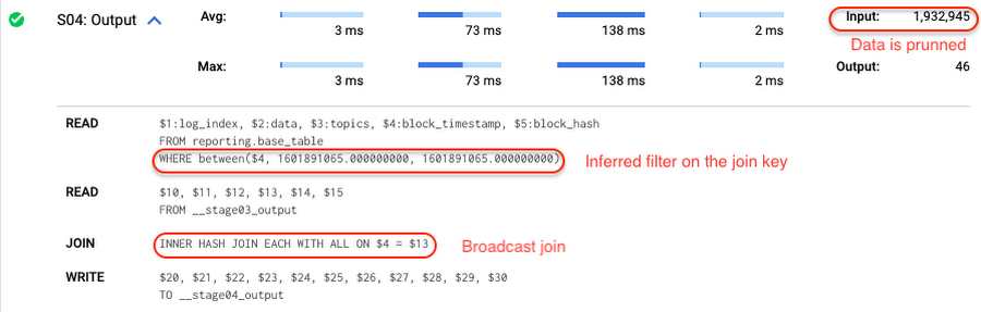
There is no requirement to join tables by partitioning or clustering key to kick off this type of optimization. However, in this case the pruning effect on the target table would be less significant.
But let us get back to the pipeline optimizations. Another way to enhance MERGE is to modify the merge_condition filter by adding static predicate on the base table:
BEGINDECLARE src_range STRUCT<date_min TIMESTAMP, date_max TIMESTAMP> --115 MB processedDEFAULT(SELECT STRUCT(MIN(block_timestamp) AS date_min,MAX(block_timestamp) AS date_max) FROM staging.load_delta);MERGE INTO reporting.base_table T --41 GB processedUSING staging.load_delta SON T.block_hash = S.block_hashAND T.log_index = S.log_indexAND T.block_timestamp BETWEEN src_range.date_min AND src_range.date_maxWHEN MATCHED THEN UPDATE SETT.data = S.dataWHEN NOT MATCHED THEN INSERT (log_index, data, topics, block_timestamp, block_hash)VALUES (log_index, data, topics, block_timestamp, block_hash);END;
To summarize, here are the steps that you can perform to enhance incremental ingestion pipelines in BigQuery. First you compute the range of updated partitions based on the small staging table. Next, you tweak the MERGE statement a bit to let BigQuery know to prune data in the base table.
All the enhanced MERGE statements scanned 41 GB of data, and setting up the src_range variable took 115 MB. Compare it with the initial 161 GB scan. Moreover, given that computing src_range may be incorporated into some existing transformation in your ETL/ELT, it results in a good performance improvement which you can leverage in your pipelines.
In this post we described how to enhance data ingestion pipelines by turning dynamic filter predicates into static predicates and letting BiQuery prune data for us. You can find more tips on BigQuery DML tuning here.
Special thanks to Daniel De Leo, who helped with examples and provided valuable feedback on this content.
Optimizing Bigtable Performance: Unveiling 20-50% Increase in Single-Row Read Throughput

1275
Of your peers have already read this article.
3:30 Minutes
The most insightful time you'll spend today!
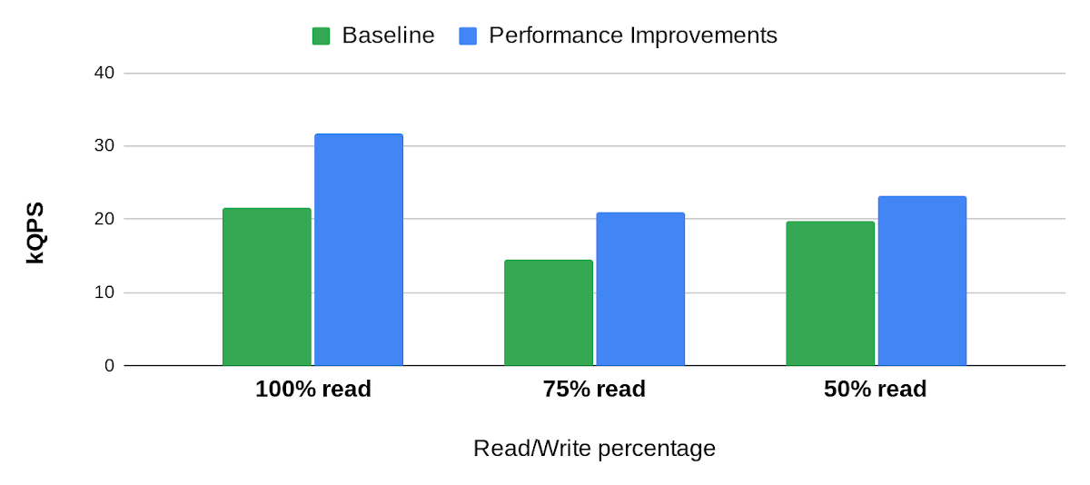
Bigtable is a scalable, distributed, high-performance NoSQL database that processes more than 6 billion requests per second at peak and has more than 10 Exabytes of data under management. Operating at this scale, Bigtable is highly optimized for high-throughput and low-latency reads and writes. Even so, our performance engineering team continually explores new areas to optimize. In this article, we share details of recent projects that helped us push Bigtable’s performance envelope forward, improving single-row read throughput by 20-50% while maintaining the same low latency.
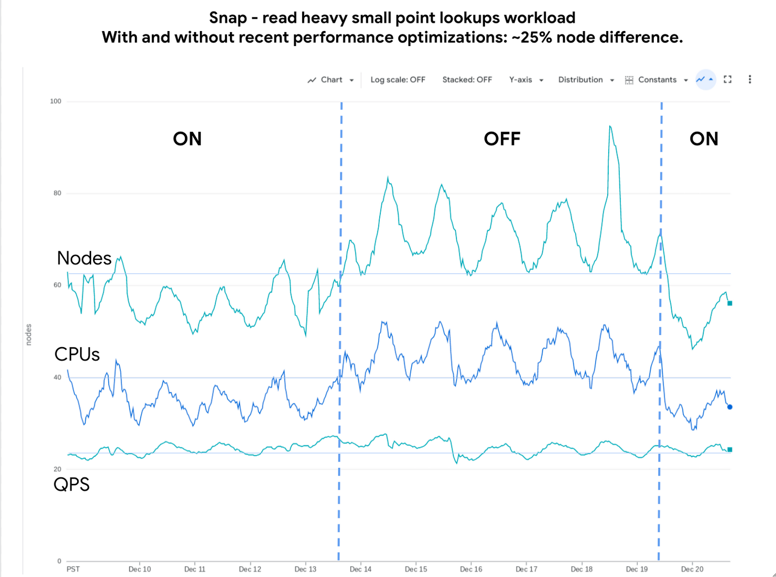
Below is an example of the impact we delivered to one of our customers, Snap. The compute cost for this small-point read-heavy workload reduced by 25% while maintaining the previous level of performance.
Performance research
We use a suite of benchmarks to continuously evaluate Bigtable’s performance. These represent a broad spectrum of workloads, access patterns and data volumes that we see across the fleet. Benchmark results give us a high-level view of performance opportunities, which we then enhance using sampling profilers and pprof for analysis. This analysis plus several iterations of prototyping confirmed feasibility of improvements in the following areas: Bloom filters, prefetching, and a new post-link-time optimization framework, Propeller.
Bloom filters
Bigtable stores its data in a log-structured merge tree. Data is organized into row ranges and each row range is represented by a set of SSTables. Each SSTable is a file that contains sorted key-value pairs. During a point-read operation, Bigtable searches across the set of SSTables to find data blocks that contain values relevant to the row-key. This is where the Bloom filter comes into play. A Bloom filter is a space-efficient probabilistic data structure that can tell whether an item is in a set, it has a small number of false positives (item may be in the set), but no false negatives (item is definitely not in the set). In Bigtable’s case, Bloom filters reduce the search area to a subset of SSTables that may contain data for a given row-key, reducing costly disk access.
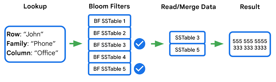
We identified two major opportunities with the existing implementation: improving utilization and reducing CPU overhead.
First, our statistics indicated that we were using Bloom filters in a lower than expected percentage of requests. This was due to our Bloom filter implementation expecting both the “column family” and the “column” in the read filter, while a high percentage of customers filter by “column family” only — which means the Bloom filter can’t be used. We increased utilization by implementing a hybrid Bloom filter that was applicable in both cases, resulting in a 4x increase in utilization. While this change made the Bloom filters larger, the overall disk footprint increased by only a fraction of a percent, as Bloom filters are typically two orders of magnitude smaller than the data they represent.
Second, the CPU cost of accessing the Bloom filters was high, so we made enhancements to Bloom filters that optimize runtime performance:
- Local cache for individual reads: When queries select multiple column families and columns in a single row, it is common that the query will use the same Bloom filter. We take advantage of this by storing a local cache of the Bloom filters used for the query being executed.
- Bloom filter index cache: Since Bloom filters are stored as data, accessing them for the first time involves fetching three blocks — two index blocks and a data block — then performing a binary search on all three. To avoid this overhead we built a custom in-memory index for just the Bloom filters. This cache tracks which Bloom filters we have in our block cache and provides direct access to them.
Overall these changes decreased the CPU cost of accessing Bloom filters by 60-70%.
Prefetching
In the previous section we noted that data for a single row may be stored in multiple SSTables. Row data from these SSTables is merged into a final result set, and because blocks can either be in memory or on disk, there’s a risk of introducing additional latency from filesystem access. Bigtable’s prefetcher was designed to read ahead of the merge logic and pull in data from disk for all SSTables in parallel.
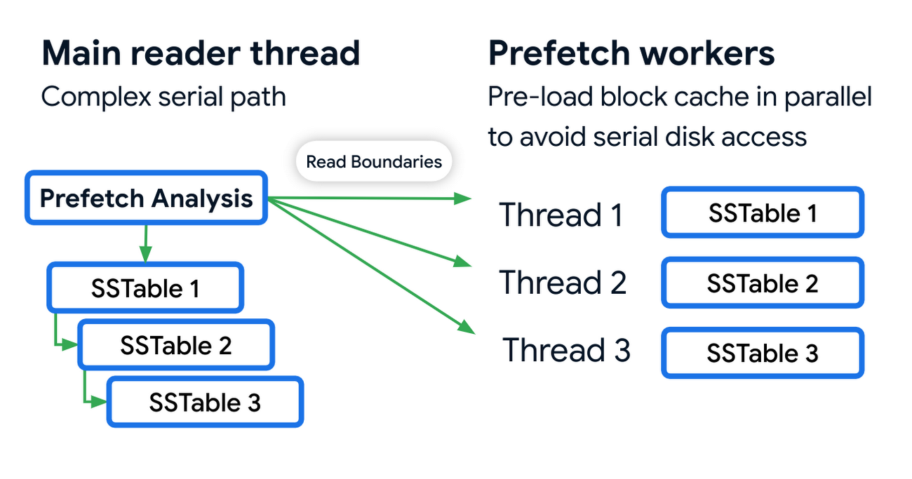
Prefetching has an associated CPU cost due to the additional threading and synchronization overhead. We reduced these costs by optimizing the prefetch threads through improved coordination with the block cache. Overall this reduced the prefetching CPU costs by almost 50%.
Post-link-time optimization
Bigtable uses profile guided optimizations (PGO) and link-time optimizations (ThinLTO). Propeller is a new post-link optimization framework released by Google that improves CPU utilization by 2-6% on top of existing optimizations.
Propeller requires additional build stages to optimize the binary. We start by building a fully optimized and annotated binary that holds additional profile mapping metadata. Then, using this annotated binary, we collected hardware profiles by running a set of training workloads that exercise critical code paths. Finally, using these profiles as input, Propeller builds a new binary with an optimized and improved code layout. Here is an example of the improved code locality.
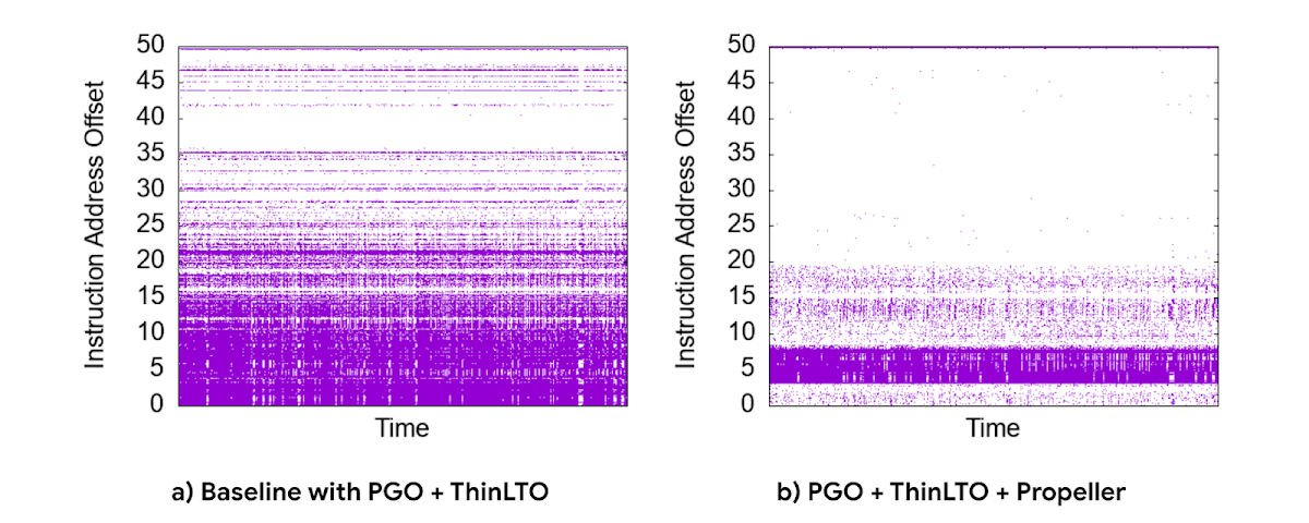
The new build process used our existing performance benchmark suite as a training workload for profile collection. The Propeller optimized binary showed promising results in our tests, showing up to 10% improvement in QPS over baseline.
However, when we released this binary to our pilot production clusters, the results were mixed. It turned out that there was overfitting for the benchmarks. We investigated sources of regression by quantifying profile overlap, inspecting hardware performance counter metrics and applied statistical analysis for noisy scenarios. To reduce overfitting, we extended our training workloads to cover a larger and more representative set of use cases.
The result was a significant improvement in CPU efficiency — reducing fleetwide utilization by 3% with an even more pronounced reduction in read-heavy workloads, where we saw up to a 10% reduction in CPU usage.
Conclusion
Overall, single-row read throughput increased by 20-50% whilst maintaining the same latency profile. We are excited about these performance gains, and continue to work on improving the performance of Bigtable. Click here to learn more about Bigtable performance and tips for testing and troubleshooting any performance issues you may encounter.
Google Introduces BigQuery Connector for SAP to Power Customers’ Data Analytics Strategy

5478
Of your peers have already read this article.
2:00 Minutes
The most insightful time you'll spend today!
Google Cloud has a genuine passion for solving technology problems that make a difference for our customers. With the release of our BigQuery Connector for SAP, we’re taking a another big step towards solving a major challenge for SAP customers with a quick, easy, and inexpensive way to integrate SAP data with BigQuery, our serverless, highly scalable, and cost-effective multi cloud data warehouse designed for business agility.
Solving for simplified data integration
Like most businesses today, SAP customers are eager to unlock the immediate insights and opportunities within their ever-growing stores of business data. However, many are discovering just how hard it can be to take the first step in any modern, cloud-enabled data analytics strategy: combining SAP data with other cloud-native, and enterprise data sets in real-time and at scale. According to a 2020 SAPInsider study, more than half of SAP customers surveyed said data integration was their top analytics pain point. These companies urgently need a rapid, sustainable, cost-effective and scalable way to integrate SAP data with modern cloud data analytics solutions.
The BigQuery Connector for SAP gives our customers a solution: a fast, simple, cost-effective and massively scalable way to make SAP data fully accessible within BigQuery by leveraging customers’ existing SAP Landscape Transformation Replication Server (SLT) tooling and skill sets. It’s the first SAP SLT direct near real-time connector for BigQuery without the need to set up additional infrastructure or third-party middleware, and can be deployed using a variety of embedded or stand-alone deployment options. In fact, most customers can install the BigQuery Connector for SAP in less than an hour—a remarkably easy way to start working with our industry-leading analytics solution that delivers proven and quantifiable business advantages for customers. Additionally, the BigQuery Connector for SAP is not restricted to customers who have deployed their SAP applications on Google Cloud. Customer’s who are running their SAP applications on-premise, or on any cloud, can also deploy and realize the analytical benefits of the solution.
Designing a solution with customer requirements and investments in mind
When the Google Cloud team started work on an analytics data integration tool for our SAP customers, we began with a set of requirements designed to root out the usual sources of cost and complexity. These included:
- The need for real-time performance with deltas replicated in milliseconds
- The ability to integrate data from almost any SAP Netweaver based application running today, regardless of its deployment location (on premises, any cloud, Google Cloud)
- Automatic BigQuery data type mapping with minimal transformation required
- Generation of target tables in BigQuery directly from source, if required
- Application layer integration that avoids the issues of direct database access
- Leveraging customers’ existing SAP skillsets, change data capture, and infrastructure
An important step towards meeting these requirements came when Alphabet, Google’s parent company, decided to leverage SAP SLT as a foundation for developing direct data replication between SAP and BigQuery for its internal corporate landscape. SLT as part of SAP’s strategic Business Technology Platform, supports real-time replication of data from SAP or third-party systems to SAP HANA, however, one of its limitations was direct integration with targets like BigQuery.
SAP SLT was a logical foundation for developing the connector for several reasons:
- It’s widely adopted among SAP customers who likely already leverage SLT for SAP analytics data integration
- It works with almost every non-SaaS SAP application environment running today
- It supports real-time replication performance at massive scale
It was an obvious choice for the Alphabet engineering team who saw immediate value from integrating SAP with BigQuery.
“The BigQuery Connector for SAP has enabled fast, low latency data replication for billions of records from 500+ tables of our most critical financial and supply chain data. Now in one cost-effective BigQuery data lake, this ERP data can be combined with other data sources for previously impossible real-time analytics and ML use cases. This allows us to drive much deeper strategic insights that support business and operational excellence, management and P&L reporting and more.”—Anil Nagalla, Sr. Engineering Director, Financial Systems, Google
SAP data integration with BigQuery enables new value
By leveraging SAP SLT, the BigQuery Connector for SAP can integrate real-time data streams from any SAP system—while also taking advantage of customers’ existing SAP investments and skillsets.
At the same time, the BigQuery Connector for SAP does a lot of heavy lifting on its own. For example, it automatically handles the complex, multi-step process of transforming SAP data types for use in BigQuery—mapping data-type transitions between the SAP and BigQuery environments, creating a target table schema on BigQuery for the transformed data types, building the target BigQuery table, and even adapting as new data types appear in your SAP environment.
For teams that want to fine-tune the BigQuery Connector for SAP’s automated recommendations, the connector supports additional levels of customization and choice. But if you simply want to get the job done and give your data analytics team greater support for their high-value work, then you’ll love just how quickly and easily the BigQuery Connector for SAP turns the complicated work of data integration and performance to process large volumes of data into a done deal. By integrating enterprise data sets in real time, customers can drive differentiated value and unlock new insights and actions that drive a competitive advantage.
The BigQuery Connector for SAP really shines as an enabling tool that transports and transforms your SAP data to power analytics solutions enabled by accelerators like the Google Cloud Cortex Framework: a comprehensive set of reference architectures, deployment accelerators, and integration services designed to give SAP customers a fast and seamless path to value with their data analytics investments. Simply put, the more SAP data you make available within Google Cloud, the easier it is to get meaningful—and often game-changing—insights from these solutions.
Learn more about the BigQuery Connector for SAP
Ready to get started with your own SAP data analytics strategy on Google Cloud? Install the Google Cloud BigQuery Connector for SAP, and discover a faster, simpler, more sustainable way to power your company’s data analytics strategy.
More Relevant Stories for Your Company

Customer Voices: How Firms from Across Industries Leverage Google Cloud
From powering everyday operations and accelerating application innovation, to providing tools for specific business needs and executing on big ideas, to advancing the security of technology solutions, companies from across industries have leveraged Google Cloud for business benefits. Companies from across industries have turned to Google Cloud for transforming their

BigQuery Explainable AI for Demystifying the Inner Workings of ML Models. Now GA!
Explainable AI (XAI) helps you understand and interpret how your machine learning models make decisions. We're excited to announce that BigQuery Explainable AI is now generally available (GA). BigQuery is the data warehouse that supports explainable AI in a most comprehensive way w.r.t both XAI methodology and model types. It does this at

Enhancing Data Governance through Automation with Dataplex and BigLake
Unlocking the full potential of data requires breaking down the silo between open-source data formats and data warehouses. At the same time, it is critical to enable data governance team to apply policies regardless of where the data happens, whether - on file or columnar storage. Today, data governance teams

Guide: Bring new life to your databases with an Oracle migration
Organizations today are being forced to make difficult decisions. Innovation has moved down the list for many companies, replaced with realities like making sure your business systems stay up and running during a disaster, managing unexpected shifts in demand,and above all, staying in business. In the short term, this means
