





Take a Look at 30 Eventrac Locations!

4924
Of your peers have already read this article.
2:00 Minutes
The most insightful time you'll spend today!
New locations in Eventarc
Back in August, we announced more Eventarc locations (17 new regions, as well as 6 new dual-region and multi-region locations to be precise). This takes the total number of locations in Eventarc to more than 30. You can see the full list in the Eventarc locations page or by running gcloud eventarc locations list .
What does location mean in Eventarc?
An Eventarc location usually refers to the single region that the Eventarc trigger gets created in. However, depending on the trigger type, the location can be more than a single region:
- Pub/Sub triggers only support single-region locations.
- Cloud Storage triggers support single-region, dual-region, and multi-region locations.
- Cloud Audit Logs triggers support single-region locations and the special
globalregion.
Before looking into trigger location in more detail, let’s look at other locations relevant in Eventarc.
What other locations are relevant in Eventarc?
Triggers connect event sources to event targets:
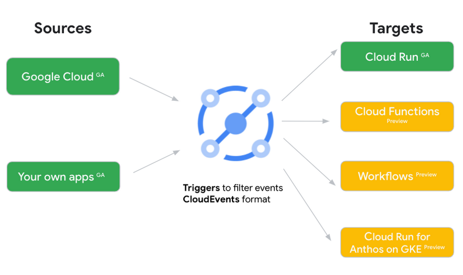
Each event source, event target, and trigger has its own location. Sometimes, these locations have to match and sometimes they can be different.
Here’s an example of a trigger connecting Cloud Storage events from a bucket in the europe-west1 region to a Cloud Run service in the us-central1 region with a trigger located in the europe-west1 region:
gcloud eventarc triggers create trigger-storage \--destination-run-service=hello \--destination-run-region=us-central1 \--location=europe-west1 \--event-filters="type=google.cloud.storage.object.v1.finalized" \--event-filters="bucket=my-bucket-in-europe-west1-region" \--service-account=$PROJECT_NUMBER-compute@developer.gserviceaccount.com
In many cases, you don’t have control over the location of the event source. In the example above, the Cloud Storage bucket is in the europe-west1 region. That’s the location that you need to work with and it has implications for the trigger location (which I’ll get to later).
The location of the event target is the region of the service where you want the events to go. You get to choose this from one of the supported regions when you deploy your Cloud Run service. You typically want this to be in the same region as your event source for latency and data locality reasons (but this is not strictly a requirement). In the example above, the event source (bucket) is in europe-west1 but the event target (Cloud Run service) is in us-central1 as specified by the --destination-run-region flag.
The location of the trigger is dictated by the event source location, but the trigger type also comes into play. It is specified by the –location flag. Let’s take a look at the trigger location for each trigger type in more detail.
Location in Pub/Sub triggers
In a Pub/Sub trigger, you connect a Pub/Sub topic to an event target. Pub/Sub topics are global and not tied to a single region. However, when you create a Pub/Sub trigger, you need to specify a region for it (because Eventarc triggers need to live in a region) with the --location flag as follows:
gcloud eventarc triggers create trigger-pubsub \--destination-run-service=hello \--destination-run-region=us-central1 \--location=us-central1 \--event-filters="type=google.cloud.pubsub.topic.v1.messagePublished" \--transport-topic=projects/your-projectid/topics/your-topic
By specifying a location, Eventarc automatically configures the geofencing feature in Pub/Sub such that events only persist in the specified location. As I noted above, you typically want to (but are not required to) choose the same region for the trigger and the Cloud Run service for lower latency and data locality. You can also use regional Pub/Sub service endpoints to publish to the topic to ensure that all of the data stays in a single region.
Location in Cloud Storage triggers
In a Cloud Storage trigger, you connect a Cloud Storage bucket to an event target. A Cloud Storage bucket can be in a single-region (e.g. europe-west1), dual-region (e.g. eur4), or multi-region (e.g. eu) location. The location of the bucket dictates the location of the trigger and they have to match. The earlier trigger example was for a bucket in the europe-west1 single-region location. Here’s another trigger connecting Cloud Storage events from a bucket in the eu multi-region location. Notice how the location flag matches the bucket region:
gcloud eventarc triggers create trigger-storage \--destination-run-service=hello \--destination-run-region=us-central1 \--location=eu \--event-filters="type=google.cloud.storage.object.v1.finalized" \--event-filters="bucket=my-bucket-in-eu-multi-region" \--service-account=$PROJECT_NUMBER-compute@developer.gserviceaccount.com
If the bucket region and the trigger region do not match, you’ll see an error:
ERROR: (gcloud.eventarc.triggers.create) INVALID_ARGUMENT: The request was invalid: Bucket "my-bucket-in-eu-multi-region" location "eu" does not match trigger location "europe-west1". Try again by creating the trigger in "eu".
Location in Cloud Audit Logs triggers
In a Cloud Audit Logs trigger, you connect any event source that emits Audit Logs to an event target. The location of the event source will dictate the trigger location. This is typically a single region but there is a special global region that’s necessary in some cases.
For example, if you want to read Cloud Storage events from a bucket in the europe-west1 region with an Audit Logs trigger, you will create the trigger with the same location. Note that this will match all buckets in the europe-west1 region as there’s no filter by bucket in Audit Logs:
gcloud eventarc triggers create trigger-auditlog \--destination-run-service=hello \--destination-run-region=us-central1 \--location=europe-west1 \--event-filters="type=google.cloud.audit.log.v1.written" \--event-filters="serviceName=storage.googleapis.com" \--event-filters="methodName=storage.objects.create" \--service-account=$PROJECT_NUMBER-compute@developer.gserviceaccount.com
On the other hand, if you want to match a dual-region or a multi-region bucket such as eu, you will create the trigger with the global location as Audit Logs triggers only support a single or global region. Note that this will match all buckets in all regions globally:
gcloud eventarc triggers create trigger-storage \--destination-run-service=hello \--destination-run-region=us-central1 \--location=global \--event-filters="type=google.cloud.storage.object.v1.finalized" \--event-filters="bucket=my-bucket-in-europe-west1-region" \--service-account=$PROJECT_NUMBER-compute@developer.gserviceaccount.com
As you can see from this example, if you want to read Cloud Storage events, the native Cloud Storage trigger is a much better option, but this example illustrates a typical case in which a global Audit Log trigger is necessary.
That wraps up this closer look at locations in Eventarc. Feel free to reach out to me on Twitter @meteatamel for any questions or feedback.
Autonom8: Achieving growth and profits for businesses with Google Cloud

3016
Of your peers have already read this article.
3:30 Minutes
The most insightful time you'll spend today!
With Google Cloud, Autonom8 can run a platform that accelerates and streamlines customer journeys in a scalable, reliable, cost-effective infrastructure, while using advanced optical character recognition to enable intelligent document processing.
About Autonom8
Headquartered in the United States and India, Autonom8 has built a low-code SaaS platform that allows businesses to digitize customer-facing workflows. The business aims to help clients reduce costs and improve interactions with their customers through automation and enablement of customer journeys.

Google Cloud results:
- Increased margins by up to 30% by switching from a home-grown OCR system to Cloud Vision AI
- Enables one DevOps team member to manage up to 30 customers
- Provides real-time information about customer journeys to enable businesses to respond quickly and accurately
- Ensures use of its platform with containerization in customers’ private data centers
- Reduced operating costs by up to 20% with localized scalability and architecture through GKE
Just as cars are evolving to become autonomous, smart and self-driving, enterprises can gain self-awareness, an ability to learn and an ability to adapt. This is the value proposition put forward by Autonom8, an India- and United States-based enterprise workflow management software business. “We provide a low-code, high-intelligence customer journey automation SaaS platform,” explains Ranjit Padmanabhan, Co-founder and Chief Technology Officer (CTO), Autonom8.
The Autonom8 platform includes components, such as A8Studio, a drag and drop location from which clients can create customer journeys, a chat platform that enables clients to create chatbots, and an analytics module. “With our platform and services, businesses can reduce costs and improve interactions with their customers by applying automation to accelerate and provide better customer journeys,” adds Padmanabhan.
Demand for Autonom8 is being driven by the changing customer demands of enterprises, including the expectation to interact with them over multiple channels, and the rising cost of building software with experienced developers. These trends place enterprises under growing pressure to increase the productivity of the people they do have, particularly those who are less technically inclined. In addition, changing consumer habits, regulations and the emergence of new technologies mean customer journeys cannot remain static and need to evolve.
Developing a microservices-based SaaS platform
From the start, Autonom8 planned to deliver a SaaS platform and initially deployed on a multinational cloud service, chosen due to the team’s familiarity with its products and the availability of credits. However, the company’s decision to opt for a microservices architecture that enables individual services to scale independently while running in a containerized environment, demanded high-quality container orchestration. To optimize cost, scalability and performance, Autonom8 began evaluating Google Kubernetes Engine (GKE).
The business then completed a side-by-side comparison between Google Cloud and its incumbent provider of compute, storage and other services. Google Cloud fared favorably, with Vision AI in particular providing powerful machine learning and optical character recognition (OCR) functionality, supporting a key use case for Autonom8.
In addition, many of Autonom8’s clients at the time are financial institutions in India, and legally required to retain data within the country’s borders. Google Cloud’s global network and local presence means the business could fulfill this requirement easily.
“We decided to evaluate Google Cloud, particularly GKE, from two perspectives. One, from a security perspective, as we sell to banks that audit our platform, and two, as a failover between regions because downtime costs money. We found it a compelling solution.”
— Ranjit Padmanabhan, Co-founder and Chief Technology Officer (CTO), Autonom8
A seamless move to Google Cloud
Autonom8 began deploying on Google Cloud in 2018, with its architecture comprising storage, compute, serverless, container management and orchestration, and Vision AI. “We looked at our scripting with the previous provider, and using the Google Cloud documentation available online, educated ourselves over a few weeks before moving pieces of our architecture step by step to Google Cloud,” says Padmanabhan. “We did not run into any major issues. It was pretty simple, with our experienced engineers training others in the product.”
According to the CTO, the business had two options when moving to Google Cloud. Autonom8 could either install raw virtual machines and effectively create its own virtualized data center, or rely on managed services for functions such as memory store, registration and authentication to save time and resources over the long term. Autonom8 opted for the latter and has transitioned fully to Google Cloud, with the number of cloud products and services in its architecture rising from five to about 15. While each product and service performs a key role in the delivery of Autonom8’s products and services, Padmanabhan nominates GKE, Vision AI and Cloud SQL as providing the greatest value to the business.
Scalability, real-time monitoring and intelligent document processing at low cost
With GKE, the business can now scale the nodes or containers specific to each microservice in the event traffic to a particular client surges, due to a rebate or promotion. “Through the combination of the architecture and localized scalability we achieve with GKE, we are reducing our operating costs by up to 20%,” says Padmanabhan.
Running an open source TimescaleDB on Postgres in Cloud SQL enables Autonom8 to give its clients the ability to monitor customer journey information in real time. An example of a journey is applying for a bank loan. The customer must take steps including providing income, tax and other financial details that the bank then appraises to help make a decision on the application. “The moment someone applies for a loan, for example, a bank knows about it and can monitor for fraud, bottlenecks, or other abnormalities, and immediately route to a remediation workflow,” explains Padmanabhan. “Cloud SQL enables us to maintain transactional logging and provide real-time data to our dashboards.”
After evaluating alternative services, including developing a home-grown OCR engine, the business turned to Cloud Vision AI to manage the intelligent document processing that comprises much of its transactional volume. “Vision AI is significantly better than the alternatives and the cost of maintaining our version did not make sense, because Google Cloud continues to make improvements over time that enable us to deliver more and more accurate results to our customers,” says Padmanabhan. “Switching from our home-grown service to Vision AI has enabled us to increase our profit margins by up to 30%.”
“Through the combination of the architecture and localized scalability we achieve with Google Kubernetes Engine, we are reducing our operating costs by up to 20%.”
—Ranjit Padmanabhan, Co-founder and Chief Technology Officer (CTO), Autonom8
Supporting client demands and improving developer efficiency
Google Cloud also enables Autonom8 to meet the demands of businesses that want to run its platform within their own private data centers. “We can undertake the build within Google Cloud and ship our containers to compatible hosts within those clients’ data centers,” explains Padmanabhan. “With our previous provider, we could create containers, but these would not run properly within those data centers.”
Furthermore, Google Cloud documentation and online resources help Autonom8 reduce the training needed for new developers to become productive, with the Google Cloud learning curve taking up just 10% of the overall onboarding cycle.
The organization spends the equivalent of just 3% of its overall annual revenue on DevOps, measured as DevOps Utility Ratio, while the cloud cost of revenue is about USD 1 for every USD 6 in annual recurring revenue, measured as Cloud Utility Ratio. “These two metrics are about what we can do with the people we have,” explains Padmanabhan. “Our current ratio implies that one DevOps person can handle approximately 30 customers. This is made possible by the tools we have, and the comprehensive support from Google Cloud in terms of security patches, intelligent alerts, resource overloading, and more.”
Google Cloud also provides the flexibility for Autonom8 to accommodate the varying service levels required by individual customers based on factors, such as the impact of downtime, as the business can failover seamlessly between regions to mitigate the impact of any issues that may occur.
“Our current ratio implies that one DevOps person can handle approximately 30 customers. This is made possible by the tools we have, and the comprehensive support from Google Cloud in terms of security patches, intelligent alerts, resource overloading, and more.”
—Ranjit Padmanabhan, Co-founder and Chief Technology Officer (CTO), Autonom8
Integrating Google Workspace with Autonom8 to deliver new capabilities
Autonom8 relies on Google Workspace for communication, collaboration and other workplace productivity requirements, growing its footprint from Gmail when the employee population was four or five, to a range of products including Sheets and Drive as the business grew. “It became natural to use the capabilities in Google Workspace as we matured,” says Padmanabhan. “One of the most interesting capabilities was our ability to integrate Google Workspace into our platform. For example, when someone is running a workflow, they can add data from a Sheet. We’ve added Google Workspace authentication capabilities into our products as well.”
“Everyone is using shared links to Drive and I really like the granular permissions structure,” he adds. “I can open up folders to clients while keeping an internal space within the business to ensure security and privacy.”
With Google Cloud, Autonom8 is now poised to continue growing its business and adding new features and capabilities for clients. “We are extremely excited at the opportunity to step up our offering to clients with Google Cloud,” concludes Padmanabhan.
Cloud Bigtable Helps Fraud-detection Company Meet Scalability Demands and Secure Customer Data

7108
Of your peers have already read this article.
3:00 Minutes
The most insightful time you'll spend today!
Editor’s note: Today we are hearing from Jono MacDougall , Principal Software Engineer at Ravelin. Ravelin delivers market-leading online fraud detection and payment acceptance solutions for online retailers. To help us meet the scaling, throughput, and latency demands of our growing roster of large-scale clients, we migrated to Google Cloud and its suite of managed services, including Cloud Bigtable, the scalable NoSQL database for large workloads.
As a fraud detection company for online retailers, each new client brings new data that must be kept in a secure manner and new financial transactions to analyze. This means our data infrastructure must be highly scalable and constantly maintain low latency. Our goal is to bring these new organizations on quickly without interrupting their business. We help our clients with checkout flows, so we need latencies that won’t interrupt that process—a critical concern in the booming online retail sector.
We like Cloud Bigtable because it can quickly and securely ingest and process a high volume of data. Our software accesses data in Bigtable every time it makes a fraud decision. When a client’s customer places an order, we need to process their full history and as much data as possible about that customer in order to detect fraud, all while keeping their data secure. Bigtable excels at accessing and processing that data in a short time window. With a customer key, we can quickly access data, bring it into our feature extraction process, and generate features for our models and rules. The data stays encrypted at rest in Bigtable, which keeps us and our customers safe.
Bigtable also lets us present customer profiles in our dashboard to our client, so that if we make a fraud decision, our clients can confirm the fraud using the same data source we use.

We have configured our bigtable clusters to only be accessible within our private network and have restricted our pods access to it using targeted service accounts. This way the majority of our code does not have access to bigtable and only the bits that do the reading and writing have those privileges.
We also use Bigtable for debugging, logging, and tracing, because we have spare capacity and it’s a fast, convenient location.
We conduct load testings against Bigtable. We started at a low rate of ~10 Bigtable requests per second and we peaked at ~167000 mixed read and write requests per second at absolute peak. The only intervention that was done to achieve this was pressing a single button to increase the number of nodes in the database. No other changes were made.
In terms of real traffic to our production system, we have seen ~22,000 req/s (combined read/write) on Bigtable in our live environment as a peak within the last 6 weeks.
Migrating seamlessly to Google Cloud
Like many startups, we started with Postgres, since it was easy and it was what we knew, but we quickly realized that scaling would be a challenge, and we didn’t want to manage enormous Postgres instances. We looked for a kind of key value store, because we weren’t doing crazy JOINS or complex WHERE clauses. We wanted to provide a customer ID and get everything we knew about it, and that’s where key value really shines.
I used Cassandra at a previous company, but we had to hire several people just for that chore. At Ravelin we wanted to move to managed services and save ourselves that headache. We were already heavy users and fans of BigQuery, Google Cloud’s serverless, scalable data warehouse, and we also wanted to start using Kubernetes. This was five years ago, and though quite a few providers offer Kubernetes services now, we still see Google Cloud at the top of that stack with Google Kubernetes Engine (GKE). We also like Bigtable’s versioning capability that helped with a use case involving upserts. All of these features helped us choose Bigtable.
Migrations can be intimidating, especially in retail where downtime isn’t an option. We were migrating not just from Postgres to Bigtable, but also from AWS to Google Cloud. To prepare, we ran in AWS like always, but at the same time we set up a queue at our API level to mirror every request over to Google Cloud. We looked at those requests to see if any were failing, and confirmed if the results and response times were the same as in AWS. We did that for a month, fine tuning along the way.
Then we took the big step and flipped a config flag and it was 100% over to Google Cloud. At the exact same time, we flipped the queue over to AWS so that we could still send traffic into our legacy environment. That way, if anything went wrong, we could fail back without missing data. We ran like that for about a month, and we never had to fail back. In the end, we pulled off a seamless, issue-free online migration to Google Cloud.
Flexing Bigtable’s features
For our database structure, we originally had everything spread across rows, and we’d use a hash of a customer ID as a prefix. Then we could scan each record of history, such as orders or transactions. But eventually we got customers that were too big, where the scanning wasn’t fast enough. So we switched and put all of the customer data into one row and the history into columns. Then each cell was a different record, order, payment method, or transaction. Now, we can quickly look up the one row and get all the necessary details of that customer. Some of our clients send us test customers who place an order, say, every minute, and that quickly becomes problematic if you want to pull out enormous amounts of data without any limits on your row size. The garbage collection feature makes it easy to clean up big customers.
We also use Bigtable replication to increase reliability, atomicity, and consistency. We need strong consistency guarantees within the context of a single request to our API since we make multiple bigtable requests within that scope. So within a request we always hit the same replica of Bigtable and if we have a failure, we retry the whole request. That allows us to make use of the replica and some of the consistency guarantees, a nice little trade-off where we can choose where we want our consistency to live.https://www.youtube.com/embed/0-eH5u7rrQQ?enablejsapi=1&
We also use BigQuery with Bigtable for training on customer records or queries with complicated WHERE clauses. We put the data in Bigtable, and also asynchronously in BigQuery using streaming inserts, which allows our data scientists to query it in every way you can imagine, build models, and investigate patterns and not worry about query engine limitations. Since our Bigtable production cluster is completely separate, doing a query on BigQuery has no impact on our response times. When we were on Postgres many years ago, it was used for both analysis and real time traffic and it was not the optimal solution for us. We also use Elasticsearch for powering text searches for our dashboard.
If you’re using Bigtable, we recommend three features:
- Key visualizer. If we get latency or errors coming back from Bigtable, we look at the key visualizer first. We may have a hotkey or a wide row, and the visualizer will alert us and provide the exact key range where the key lives, or the row in question. Then we can go in and fix it at that level. It’s useful to know how your data is hitting Bigtable and if you’re using any anti-patterns or if your clients have changed their traffic pattern that exacerbated some issue.
- Garbage collection. We can prevent big row issues by putting size limits in place with the garbage collection policies.
- Cell versioning. Bigtable has a 3d array, with rows, columns, and cells, which are all the different versions. You can make use of the versioning to get history of a particular value or to build a time series within one row. Getting a single row is very fast in Bigtable so as long as you can keep the data volume in check for that row, making use of cell versions is a very powerful and fast option. There are patterns in the docs that are quite useful and not immediately obvious. For example, one trick is to reverse your timestamps (MAXINT64 – now) so instead of the latest version, you can get the oldest version effectively reversing the cell version sorting if you need it.
Google Cloud and Bigtable help us meet the low-latency demands of the growing online retail sector, with speed and easy integration with other Google Cloud services like BigQuery. With their managed services, we freed up time to focus on innovations and meet the needs of bigger and bigger customers.
Learn more about Ravelin and Bigtable, and check out our recent blog, How BIG is Cloud Bigtable?
10151
Of your peers have already watched this video.
1:00 Minutes
The most insightful time you'll spend today!
Predict User Churn on Gaming Apps with Google Analytics Data using BigQuery ML
User retention can be a major challenge for mobile game developers. According to the Mobile Gaming Industry Analysis in 2019, most mobile games only see a 25% retention rate for users after the first day. To retain a larger percentage of users after their first use of an app, developers can take steps to motivate and incentivize certain users to return. But to do so, developers need to identify the propensity of any specific user returning after the first 24 hours.
In this blog post, we will discuss how you can use BigQuery ML to run propensity models on Google Analytics 4 data from your gaming app to determine the likelihood of specific users returning to your app.
You can also use the same end-to-end solution approach in other types of apps using Google Analytics for Firebase as well as apps and websites using Google Analytics 4. To try out the steps in this blogpost or to implement the solution for your own data, you can use this Jupyter Notebook.
Using this blog post and the accompanying Jupyter Notebook, you’ll learn how to:
- Explore the BigQuery export dataset for Google Analytics 4
- Prepare the training data using demographic and behavioural attributes
- Train propensity models using BigQuery ML
- Evaluate BigQuery ML models
- Make predictions using the BigQuery ML models
- Implement model insights in practical implementations
Google Analytics 4 (GA4) properties unify app and website measurement on a single platform and are now default in Google Analytics. Any business that wants to measure their website, app, or both, can use GA4 for a more complete view of how customers engage with their business. With the launch of Google Analytics 4, BigQuery export of Google Analytics data is now available to all users. If you are already using a Google Analytics 4 property, you can follow this guide to set up exporting your GA data to BigQuery.
Once you have set up the BigQuery export, you can explore the data in BigQuery. Google Analytics 4 uses an event-based measurement model. Each row in the data is an event with additional parameters and properties. The Schema for BigQuery Export can help you to understand the structure of the data.
In this blogpost, we use the public sample export data from an actual mobile game app called “Flood It!” (Android, iOS) to build a churn prediction model. But you can use data from your own app or website.
Here’s what the data looks like. Each row in the dataset is a unique event, which can contain nested fields for event parameters.
SELECT *FROM `firebase-public-project.analytics_153293282.events_*`TABLESAMPLE SYSTEM (1 PERCENT)
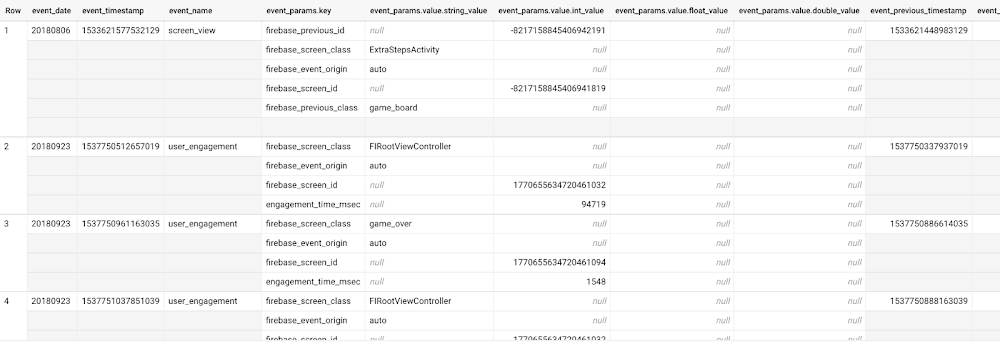
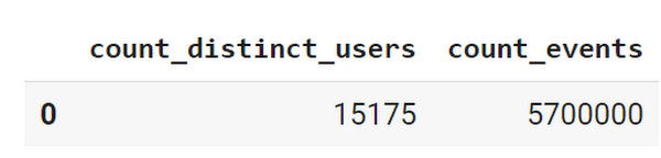
This dataset contains 5.7M events from over 15k users.
SELECTCOUNT(DISTINCT user_pseudo_id) as count_distinct_users,COUNT(event_timestamp) as count_eventsFROM`firebase-public-project.analytics_153293282.events_*
Our goal is to use BigQuery ML on the sample app dataset to predict propensity to user churn or not churn based on users’ demographics and activities within the first 24 hours of app installation.
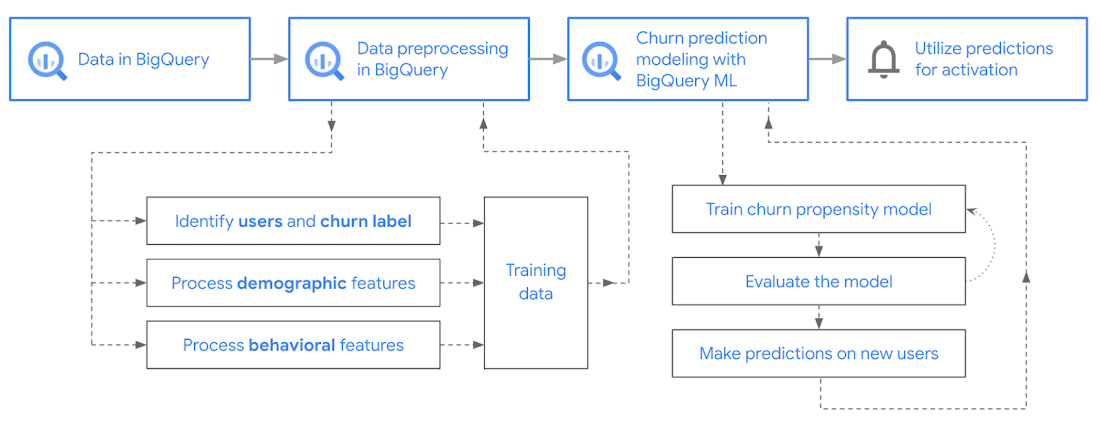
In the following sections, we’ll cover how to:
- Pre-process the raw event data from GA4
- Identify users & the label feature
- Process demographic features
- Process behavioral features
- Train classification model using BigQuery ML
- Evaluate the model using BigQueryML
- Make predictions using BigQuery ML
- Utilize predictions for activation
Pre-process the raw event data
You cannot simply use raw event data to train a machine learning model as it would not be in the right shape and format to use as training data. So in this section, we’ll go through how to pre-process the raw data into an appropriate format to use as training data for classification models.
This is what the training data should look like for our use case at the end of this section:
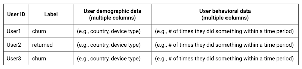
Notice that in this training data, each row represents a unique user with a distinct user ID (user_pseudo_id).
Identify users & the label feature
We first filtered the dataset to remove users who were unlikely to return the app anyway. We defined these ‘bounced’ users as ones who spent less than 10 mins with the app. Then we labeled all remaining users:
- churned: No event data for the user after 24 hours of first engaging with the app.
- returned: The user has at least one event record after 24 hours of first engaging with the app.
For your use case, you can have a different definition of bounce and churning. Also you can even try to predict something else other than churning, e.g.:
- whether a user is likely to spend money on in-game currency
- likelihood of completing n-number of game levels
- likelihood of spending n amount of time in-game etc.
In such cases, label each record accordingly so that whatever you are trying to predict can be identified from the label column.
From our dataset, we found that ~41% users (5,557) bounced. However, from the remaining users (8,031), ~23% (1,883) churned after 24 hours:
SELECTbounced,churned,COUNT(churned) as count_usersFROMbqmlga4.returningusersGROUP BY 1,2ORDER BY bounced
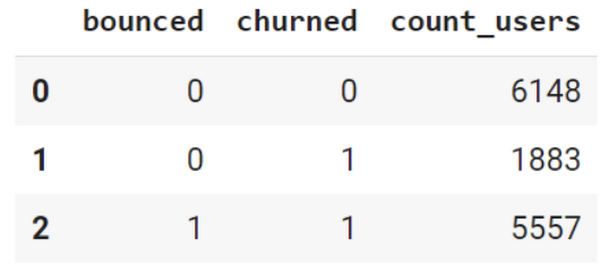
To create these bounced and churned columns, we used the following snippet of SQL code.
...#churned = 1 if last_touch within 24 hr of app installation, else 0IF (user_last_engagement < TIMESTAMP_ADD(user_first_engagement,INTERVAL 24 HOUR),1,0 ) AS churned,#bounced = 1 if last_touch within 10 min, else 0IF (user_last_engagement <= TIMESTAMP_ADD(user_first_engagement,INTERVAL 10 MINUTE),1,0 ) AS bounced,...
You can view the Jupyter Notebook for the full query used for materializing the bounced and churned labels.
Process demographic features
Next, we added features both for demographic data and for behavioral data spanning across multiple columns. Having a combination of both demographic data and behavioral data helps to create a more predictive model.
We used the following fields for each user as demographic features:
geo.countrydevice.operating_systemdevice.language
A user might have multiple unique values in these fields — for example if a user uses the app from two different devices. To simplify, we used the values from the very first user engagement event.
CREATE OR REPLACE VIEW bqmlga4.user_demographics AS (WITH first_values AS (SELECTuser_pseudo_id,geo.country as country,device.operating_system as operating_system,device.language as language,ROW_NUMBER() OVER (PARTITION BY user_pseudo_id ORDER BY event_timestamp DESC) AS row_numFROM `firebase-public-project.analytics_153293282.events_*`WHERE event_name="user_engagement")SELECT * EXCEPT (row_num)FROM first_valuesWHERE row_num = 1 #first engagement);
Process behavioral features
There is additional demographic information present in the GA4 export dataset, e.g. app_info, device, event_params, geo etc. You may also send demographic information to Google Analytics through each hit via user_properties. Furthermore, if you have first-party data on your own system, you can join that with the GA4 export data based on user_ids.
To extract user behavior from the data, we looked into the user’s activities within the first 24 hours of first user engagement. In addition to the events automatically collected by Google Analytics, there are also the recommended events for games that can be explored to analyze user behavior. For our use case, to predict user churn, we counted the number of times the follow events were collected for a user within 24 hours of first user engagement:
user_engagementlevel_start_quickplaylevel_end_quickplaylevel_complete_quickplaylevel_reset_quickplaypost_scorespend_virtual_currencyad_rewardchallenge_a_friendcompleted_5_levelsuse_extra_steps
The following query shows how these features were calculated:
WITHevents_first24hr AS (SELECTe.*FROM`firebase-public-project.analytics_153293282.events_*` eJOINbqmlga4.returningusers rONe.user_pseudo_id = r.user_pseudo_idWHERETIMESTAMP_MICROS(e.event_timestamp) <= r.ts_24hr_after_first_engagement)SELECTuser_pseudo_id,SUM(IF(event_name = 'user_engagement', 1, 0)) AS cnt_user_engagement,# ... repeated for all behavior data ...SUM(IF(event_name = 'use_extra_steps', 1, 0)) AS cnt_use_extra_steps,FROMevents_first24hrGROUP BY1
View the notebook for the query used to aggregate and extract the behavioral data. You can use different sets of events for your use case. To view the complete list of events, use the following query:
SELECTevent_name,COUNT(event_name) as event_countFROM`firebase-public-project.analytics_153293282.events_*`GROUP BY 1ORDER BYevent_count DESC
After this we combined the features to ensure our training dataset reflects the intended structure. We had the following columns in our table:
- User ID:
user_pseudo_id
- Label:
churned
- Demographic features
countrydevice_osdevice_language
- Behavioral features
cnt_user_engagementcnt_level_start_quickplaycnt_level_end_quickplaycnt_level_complete_quickplaycnt_level_reset_quickplaycnt_post_scorecnt_spend_virtual_currencycnt_ad_rewardcnt_challenge_a_friendcnt_completed_5_levelscnt_use_extra_stepsuser_first_engagement
At this point, the dataset was ready to train the classification machine learning model in BigQuery ML. Once trained, the model will output a propensity score between churn (churned=1) or return (churned=0) indicating the probability of a user churning based on the training data.
Train classification model
When using the CREATE MODEL statement, BigQuery ML automatically splits the data between training and test. Thus the model can be evaluated immediately after training (see the documentation for more information).
For the ML model, we can choose among the following classification algorithms where each type has its own pros and cons:
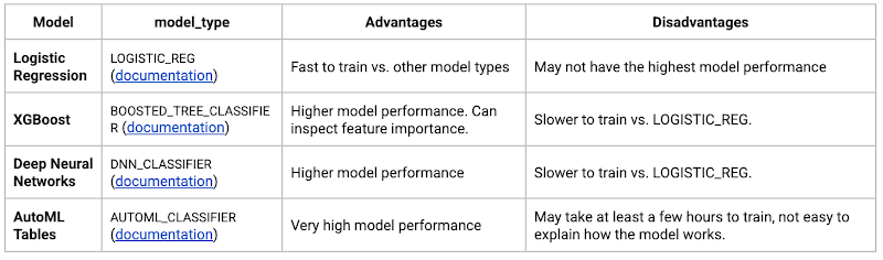
Often logistic regression is used as a starting point because it is the fastest to train. The query below shows how we trained the logistic regression classification models in BigQuery ML.
CREATE OR REPLACE MODEL bqmlga4.churn_logregTRANSFORM(EXTRACT(MONTH from user_first_engagement) as month,EXTRACT(DAYOFYEAR from user_first_engagement) as julianday,EXTRACT(DAYOFWEEK from user_first_engagement) as dayofweek,EXTRACT(HOUR from user_first_engagement) as hour,* EXCEPT(user_first_engagement, user_pseudo_id))OPTIONS(MODEL_TYPE="LOGISTIC_REG",INPUT_LABEL_COLS=["churned"]) ASSELECT*FROMbqmlga4.train
We extracted month, julianday, and dayofweek from datetimes/timestamps as one simple example of additional feature preprocessing before training. Using TRANSFORM() in your CREATE MODEL query allows the model to remember the extracted values. Thus, when making predictions using the model later on, these values won’t have to be extracted again. View the notebook for the example queries to train other types of models (XGBoost, deep neural network, AutoML Tables).
Evaluate model
Once the model finished training, we ran ML.EVALUATE to generate precision, recall, accuracy and f1_score for the model:
SELECT*FROMML.EVALUATE(MODEL bqmlga4.churn_logreg)

The optional THRESHOLD parameter can be used to modify the default classification threshold of 0.5. For more information on these metrics, you can read through the definitions on precision and recall, accuracy, f1-score, log_loss and roc_auc. Comparing the resulting evaluation metrics can help to decide among multiple models.Furthermore, we used a confusion matrix to inspect how well the model predicted the labels, compared to the actual labels. The confusion matrix is created using the default threshold of 0.5, which you may want to adjust to optimize for recall, precision, or a balance (more information here).
SELECTexpected_label,_0 AS predicted_0,_1 AS predicted_1FROMML.CONFUSION_MATRIX(MODEL bqmlga4.churn_logreg)
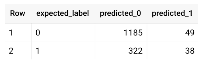
This table can be interpreted in the following way:

Make predictions using BigQuery ML
Once the ideal model was available, we ran ML.PREDICT to make predictions. For propensity modeling, the most important output is the probability of a behavior occurring. The following query returns the probability that the user will return after 24 hrs. The higher the probability and closer it is to 1, the more likely the user is predicted to return, and the closer it is to 0, the more likely the user is predicted to churn.
SELECTuser_pseudo_id,returned,predicted_returned,predicted_returned_probs[OFFSET(0)].prob as probability_returnedFROMML.PREDICT(MODEL bqmlga4.churn_logreg,(SELECT * FROM bqmlga4.train)) #can be replaced with a proper test dataset
Utilize predictions for activation
Once the model predictions are available for your users, you can activate this insight in different ways. In our analysis, we used user_pseudo_id as the user identifier. However, ideally, your app should send back the user_id from your app to Google Analytics. In addition to using first-party data for model predictions, this will also let you join back the predictions from the model into your own data.
- You can import the model predictions back into Google Analytics as a user attribute. This can be done using the Data Import feature for Google Analytics 4. Based on the prediction values you can Create and edit audiences and also do Audience targeting. For example, an audience can be users with prediction probability between 0.4 and 0.7, to represent users who are predicted to be “on the fence” between churning and returning.
- For Firebase Apps, you can use the Import segments feature. You can tailor user experience by targeting your identified users through Firebase services such as Remote Config, Cloud Messaging, and In-App Messaging. This will involve importing the segment data from BigQuery into Firebase. After that you can send notifications to the users, configure the app for them, or follow the user journeys across devices.
- Run targeted marketing campaigns via CRMs like Salesforce, e.g. send out reminder emails.
You can find all of the code used in this blogpost in the Github repository:
What’s next?
Continuous model evaluation and re-training
As you collect more data from your users, you may want to regularly evaluate your model on fresh data and re-train the model if you notice that the model quality is decaying.
Continuous evaluation—the process of ensuring a production machine learning model is still performing well on new data—is an essential part in any ML workflow. Performing continuous evaluation can help you catch model drift, a phenomenon that occurs when the data used to train your model no longer reflects the current environment.
To learn more about how to do continuous model evaluation and re-train models, you can read the blogpost: Continuous model evaluation with BigQuery ML, Stored Procedures, and Cloud Scheduler
More resources
If you’d like to learn more about any of the topics covered in this post, check out these resources:
- BigQuery export of Google Analytics data
- BigQuery ML quickstart
- Events automatically collected by Google Analytics 4
- Qwiklabs: Create ML models with BigQuery ML
Or learn more about how you can use BigQuery ML to easily build other machine learning solutions:
- How to build demand forecasting models with BigQuery ML
- How to build a recommendation system on e-commerce data using BigQuery ML
Let us know what you thought of this post, and if you have topics you’d like to see covered in the future! You can find us on Twitter at @polonglin and @_mkazi_.Thanks to reviewers: Abhishek Kashyap, Breen Baker, David Sabater Dinter.

3480
Of your peers have already downloaded this article
1:30 Minutes
The most insightful time you'll spend today!
Reduce risks, increase uptime, and free up working capital with Google Cloud’s SAP Business Continuity Program. Working closely with our experienced partner community, we will ease the lift and shift of your on premises or hosted SAP environments with simple, no-cost migrations.
Gain a future-proof digital business platform with integrated artificial intelligence, machine learning, and advanced analytics that deliver deep insights for all who need them.
Get the performance, compute power, flexibility, scalability, availability, and security you need for your current and future business needs with SAP on Google Cloud. Download this factsheet to learn more.

Gartner Names Google Cloud a Leader in the 2019 Cloud Infrastructure as a Service Market
DOWNLOAD WHITEPAPER3536
Of your peers have already downloaded this article
2:30 Minutes
The most insightful time you'll spend today!
As increasing amount of cloud IaaS is being bought for traditional IT, with an emphasis on cost reduction, safety and security, service providers are offering a high-quality service, with excellent availability, good performance, high security and good customer support.
In its Magic Quadrant for Cloud Infrastructure as a Service (IaaS), Gartner notes that the distinctions among providers are apparent in the market for cloud IaaS in terms of worldwide enterprise adoption, capabilities and service availability. Infrastructure and operations leaders should evaluate providers with broad capabilities and a positive track record for customer success.
Download the Gartner Magic Quadrant to understand why Google is a leader in the market.
More Relevant Stories for Your Company

Total Economic Impact of Running SAP on Google Cloud: Forrester’s Report
Forrester interviewed 6 customers, conducted a survey as well as a data aggregation to measure the total economic impact of running and migrating SAP systems on Google Cloud. Download the report for details on the findings on the benefits and three-year financial impact!

Google Cloud Garners Highest Score in Forrester New Wave for Computer Vision Platforms
In Forrester's evaluation of the emerging market for computer vision platforms, it identified the 11 most significant providers in the category — Amazon Web Services, Chooch AI, Clarifai, Deepomatic, EdgeVerve, Google, Hive, IBM, Microsoft, Neurala, and SAS — and evaluated them. Its report details its findings about how well each
How We Built a Brand New Bank on Google Cloud and Cloud Spanner: The First Scalable, Enterprise-grade, Database Service
Editor’s note: Technology today lets companies of any size take on entire industries simply with an innovative business model plus digital distribution. Take Shine, a French startup whose platform helps freelancers manage their finances -- and their administrative commitments. Here, Raphael Simon, Shine’s CTO and co-founder, talks about why Shine



HSBC Looks to Google Cloud to Transform Banking
HSBC, a global bank that is a central part of global commerce with a presence in 67 countries, serving 38 million customers ranging from individuals to small businesses to corporations and governments, and having over $2.5 trillion assets in its balance sheet, had a vision of being a cloud first
