When it comes to anomaly detection, one of the key challenges that many organizations face is that it can be difficult to know how to define what an anomaly is. How do you define and anticipate unusual network intrusions, manufacturing defects, or insurance fraud? If you have labeled data with known anomalies, then you can choose from a variety of supervised machine learning model types that are already supported in BigQuery ML. But what can you do if you don’t know what kind of anomaly to expect, and you don’t have labeled data? Unlike typical predictive techniques that leverage supervised learning, organizations may need to be able to detect anomalies in the absence of labeled data. 

Today we are announcing the public preview of new anomaly detection capabilities in BigQuery ML that leverage unsupervised machine learning to help you detect anomalies without needing labeled data. Depending on whether or not the training data is time series, users can now detect anomalies in training data or on new input data using a new ML.DETECT_ANOMALIES function (documentation), with the following models:

• Autoencoder model, now in Public Preview (documentation)
• K-means model, already GA (documentation)
• ARIMA_PLUS time series model, already GA (documentation)

How does anomaly detection with ML.DETECT_ANOMALIES work?

To detect anomalies in non-time-series data, you can use:

• K-means clustering models: When you use ML.DETECT_ANOMALIES with a k-means model, anomalies are identified based on the value of each input data point’s normalized distance to its nearest cluster. If that distance exceeds a threshold determined by the contamination value provided by the user, the data point is identified as an anomaly. 
• Autoencoder models: When you use ML.DETECT_ANOMALIES with an autoencoder model, anomalies are identified based on the reconstruction error for each data point. If the error exceeds a threshold determined by the contamination value, it is identified as an anomaly. 

To detect anomalies in time-series data, you can use: 

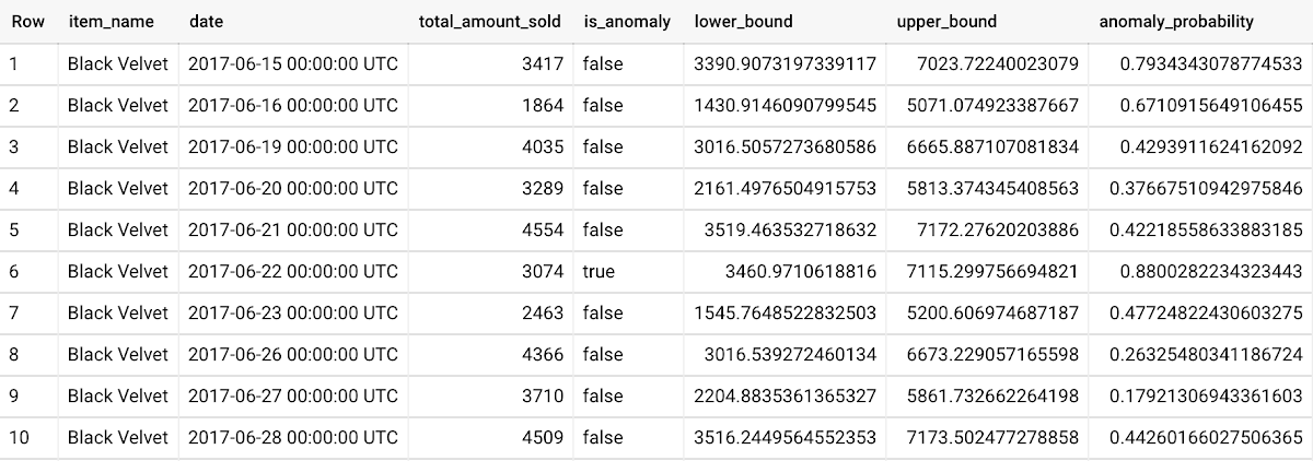
• ARIMA_PLUS time series models: When you use ML.DETECT_ANOMALIES with an ARIMA_PLUS model, anomalies are identified based on the confidence interval for that timestamp. If the probability that the data point at that timestamp occurs outside of the prediction interval exceeds a probability threshold provided by the user, the datapoint is identified as an anomaly.

Below we show code examples of anomaly detection in BigQuery ML for each of the above scenarios.

Anomaly detection with a k-means clustering model

You can now detect anomalies using k-means clustering models, by running ML.DETECT_ANOMALIES to detect anomalies in the training data or in new input data. Begin by creating a k-means clustering model:

Language: SQL

  CREATE MODEL `mydataset.my_kmeans_model`
OPTIONS(
  MODEL_TYPE = 'kmeans',
  NUM_CLUSTERS = 8,
  KMEANS_INIT_METHOD = 'kmeans++'
) AS
SELECT 
  * EXCEPT(Time, Class) 
FROM 
  `bigquery-public-data.ml_datasets.ulb_fraud_detection`;

With the k-means clustering model trained, you can now run ML.DETECT_ANOMALIES to detect anomalies in the training data or in new input data.
To detect anomalies in the training data, use ML.DETECT_ANOMALIES with the same data used during training:

Language: SQL

  SELECT
  *
FROM
  ML.DETECT_ANOMALIES(MODEL `mydataset.my_kmeans_model`,
                      STRUCT(0.02 AS contamination),
                      TABLE `bigquery-public-data.ml_datasets.ulb_fraud_detection`);

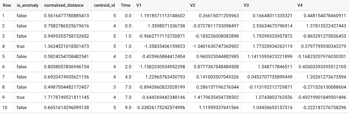
To detect anomalies in new data, use ML.DETECT_ANOMALIES and provide new data as input:

Language: SQL

  SELECT
  *
FROM
  ML.DETECT_ANOMALIES(MODEL `mydataset.my_kmeans_model`,
                      STRUCT(0.02 AS contamination),
                      (SELECT * FROM `mydataset.newdata`));

How does anomaly detection work for k-means clustering models? 

Anomalies are identified based on the value of each input data point’s normalized distance to its nearest cluster, which, if exceeds a threshold determined by the contamination value, is identified as an anomaly. How does this work exactly? With a k-means model and data as inputs, ML.DETECT_ANOMALIES first computes the absolute distance for each input data point to all cluster centroids in the model, then normalizes each distance by the respective cluster radius (which is defined as the standard deviation of the absolute distances of all points in this cluster to the centroid). For each data point, ML.DETECT_ANOMALIES returns the nearest centroid_id based on normalized_distance, as seen in the screenshot above. The contamination value, specified by the user, determines the threshold of whether a data point is considered an anomaly. For example, a contamination value of 0.1 means that the top 10% of descending normalized distance from the training data will be used as the cut-off threshold. If the normalized distance for a datapoint exceeds the threshold, then it is identified as an anomaly. Setting an appropriate contamination will be highly dependent on the requirements of the user or business. 

For more information on anomaly detection with k-means clustering, please see the documentation here.

Anomaly detection with an autoencoder model

You can now detect anomalies using autoencoder models, by running ML.DETECT_ANOMALIES to detect anomalies in the training data or in new input data. 

Begin by creating an autoencoder model:

Language: SQL

  CREATE MODEL `mydataset.my_autoencoder_model`
OPTIONS(
  model_type='autoencoder',
  activation_fn='relu',
  batch_size=8,
  dropout=0.2,  
  hidden_units=[32, 16, 4, 16, 32],
  learn_rate=0.001,
  l1_reg_activation=0.0001,
  max_iterations=10,
  optimizer='adam'
) AS 
SELECT 
  * EXCEPT(Time, Class) 
FROM 
  `bigquery-public-data.ml_datasets.ulb_fraud_detection`;

To detect anomalies in the training data, use ML.DETECT_ANOMALIES with  the same data used during training:

Language: SQL

  SELECT
  *
FROM
  ML.DETECT_ANOMALIES(MODEL `mydataset.my_autoencoder_model`,
                      STRUCT(0.02 AS contamination),
                      TABLE `bigquery-public-data.ml_datasets.ulb_fraud_detection`);

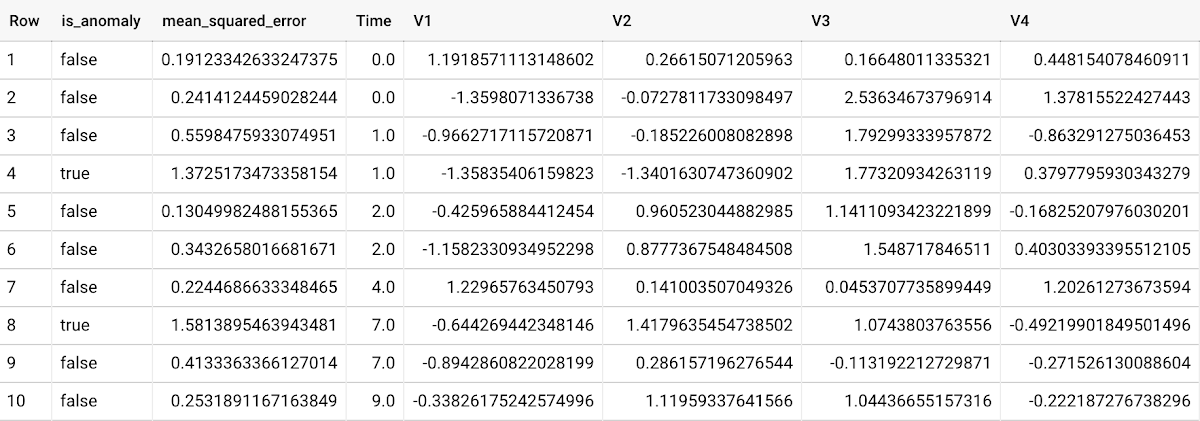
To detect anomalies in new data, use ML.DETECT_ANOMALIES and provide new data as input:

Language: SQL

  SELECT
  *
FROM
  ML.DETECT_ANOMALIES(MODEL `mydataset.my_autoencoder_model`,
                      STRUCT(0.02 AS contamination),
                      (SELECT * FROM `mydataset.newdata`));

How does anomaly detection work for autoencoder models? 

Anomalies are identified based on the value of each input data point’s reconstructed error, which, if exceeds a threshold determined by the contamination value, is identified as an anomaly. How does this work exactly? With an autoencoder model and data as inputs, ML.DETECT_ANOMALIES first computes the mean_squared_error for each data point between its original values and its reconstructed values. The contamination value, specified by the user, determines the threshold of whether a data point is considered an anomaly. For example, a contamination value of 0.1 means that the top 10% of descending error from the training data will be used as the cut-off threshold. Setting an appropriate contamination will be highly dependent on the requirements of the user or business. 

For more information on anomaly detection with autoencoder models, please see the documentation here.

Anomaly detection with an ARIMA_PLUS time-series model

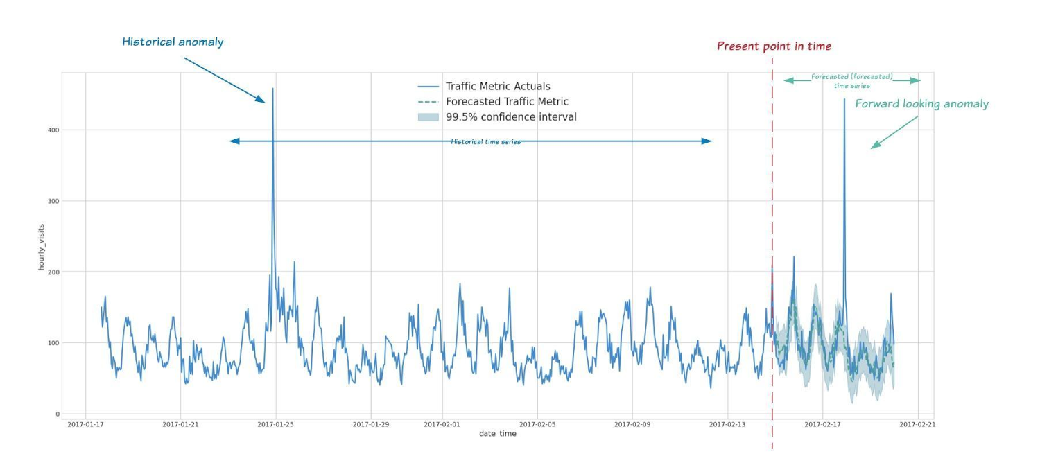
With ML.DETECT_ANOMALIES, you can now detect anomalies using ARIMA_PLUS time series models in the (historical) training data or in new input data. Here are some examples of when might you want to detect anomalies with time-series data:

Detecting anomalies in historical data: 

• Cleaning up data for forecasting and modeling purposes, e.g. preprocessing historical time series before using them to train an ML model.  
• When you have a large number of retail demand time series (thousands of products across hundreds of stores or zip codes), you may want to quickly identify which stores and product categories had anomalous sales patterns, and then perform a deeper analysis of why that was the case.

Forward looking anomaly detection: 

• Detecting consumer behavior and pricing anomalies as early as possible: e.g. if traffic to a specific product page suddenly and unexpectedly spikes, it might be because of an error in the pricing process that leads to an unusually low price. 
• When you have a large number of retail demand time series (thousands of products across hundreds of stores or zip codes), you would like to identify which stores and product categories had anomalous sales patterns based on your forecasts, so you can quickly respond to any unexpected spikes or dips.

How do you detect anomalies using ARIMA_PLUS? Begin by creating an ARIMA_PLUS time series model:

Language: SQL

  CREATE OR REPLACE MODEL mydataset.my_arima_plus_model
OPTIONS(
  MODEL_TYPE='ARIMA_PLUS',
  TIME_SERIES_TIMESTAMP_COL='date',
  TIME_SERIES_DATA_COL='total_amount_sold',
  TIME_SERIES_ID_COL='item_name',
  HOLIDAY_REGION='US' 
) AS
SELECT
  date,
  item_description AS item_name,
  SUM(bottles_sold) AS total_amount_sold
FROM
  `bigquery-public-data.iowa_liquor_sales.sales`
GROUP BY
  date,
  item_name
HAVING
  date BETWEEN DATE('2016-01-04') AND DATE('2017-06-01')
  AND item_name IN ("Black Velvet", "Captain Morgan Spiced Rum",
    "Hawkeye Vodka", "Five O'Clock Vodka", "Fireball Cinnamon Whiskey");

To detect anomalies in the training data, use ML.DETECT_ANOMALIES with the model obtained above:

Language: SQL

  SELECT
  *
FROM
  ML.DETECT_ANOMALIES(MODEL `mydataset.my_arima_plus_model`,
                      STRUCT(0.8 AS anomaly_prob_threshold));

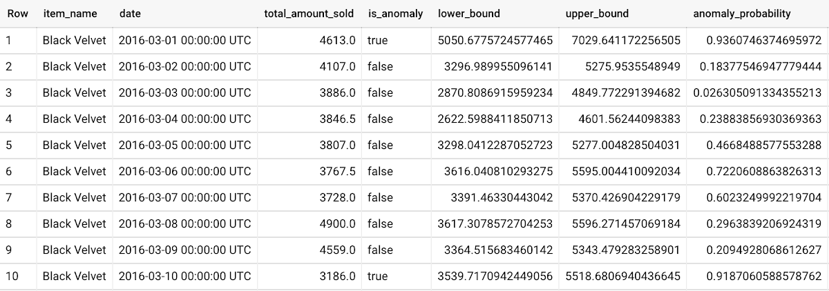
To detect anomalies in new data, use ML.DETECT_ANOMALIES and provide new data as input:

Language: SQL

  WITH
  new_data AS (
  SELECT
    date,
    item_description AS item_name,
    SUM(bottles_sold) AS total_amount_sold
  FROM
    `bigquery-public-data.iowa_liquor_sales.sales`
  GROUP BY
    date,
    item_name
  HAVING
    date BETWEEN DATE('2017-06-02')
    AND DATE('2017-10-01')
    AND item_name IN ('Black Velvet',
      'Captain Morgan Spiced Rum',
      'Hawkeye Vodka',
      "Five O'Clock Vodka",
      'Fireball Cinnamon Whiskey') )
SELECT
  *
FROM
  ML.DETECT_ANOMALIES(MODEL `mydataset.my_arima_plus_model`,
    STRUCT(0.8 AS anomaly_prob_threshold),
    (SELECT
      *
    FROM
      new_data));

For more information on anomaly detection with ARIMA_PLUS time series models, please see the documentation here.

Thanks to the BigQuery ML team, especially Abhinav Khushraj, Abhishek Kashyap, Amir Hormati, Jerry Ye, Xi Cheng, Skander Hannachi, Steve Walker, and Stephanie Wang.

At Google Cloud, we believe you get most benefits from the cloud when you scale infrastructure based on changing demand. Compute Engine allows you to configure autoscaling to save costs during periods of low demand, and add capacity to support peak loads. 

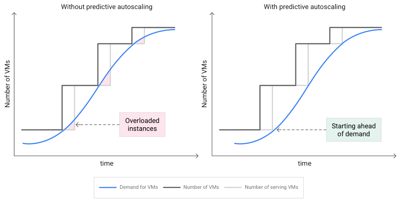
When you use a managed instance group (MIG), you can have an autoscaler automatically create or delete virtual machine (VM) instances based on increases or decreases in load. However, if your application takes several minutes to initialize, creating VMs in response to growing load might not increase your application’s capacity quickly enough. For example, if there’s a large increase in load (like when users first wake up in the morning), some users might experience delays while your application is initializing on new instances.

A good way to solve this problem would be to create VMs ahead of demand so that your application has enough time to initialize beforehand. This requires knowing upcoming demand. If only we could predict the future… Well, now we can!

Introducing predictive autoscaling

Predictive autoscaling uses Google Cloud’s machine learning capabilities to forecast capacity needs. It creates VMs ahead of growing demand allowing enough time for your application to initialize.

How does it work?

Predictive autoscaling uses your instance group’s CPU history to forecast future load and calculate how many VMs are needed to meet your target CPU utilization. Our machine learning adjusts the forecast based on recurring load patterns for each MIG. 

You can specify how far in advance you want autoscaler to create new VMs by configuring the application initialization period. For example, if your app takes 5 minutes to initialize, autoscaler will create new instances 5 minutes ahead of the anticipated load increase. This allows you to keep your CPU utilization within the target and keep your application responsive even when there’s high growth in demand. 

Many of our customers have different capacity needs during different times of the day or different days of the week. Our forecasting model understands weekly and daily patterns to cover for these differences. For example, if your app usually needs less capacity on the weekend our forecast will capture that. Or, if you have higher capacity needs during working hours, we also have you covered.

Why should you try it?

Predictive autoscaling continuously adapts forecasted capacity to best match upcoming demand. Autoscaler checks the forecast several times per minute and creates or deletes VMs to match its prediction. The forecast itself is updated every few minutes to match recent load trends so if your growth rate is higher or lower than usual we will adjust the forecast accordingly. This gives you capacity needed to cover peak load while saving on cost when demand goes down. 

You can start using predictive autoscaling without worry as it’s fully compatible with the current autoscaler. Autoscaler will calculate enough VMs to cover both forecasted as well as real-time CPU load—whichever is higher. This works with other autoscaling features as well: you can scale based on schedule, your Load Balancer request target or Cloud Monitoring metrics. Autoscaler provides enough capacity to all of your configurations by taking the highest number of VMs needed to meet all your targets.

Getting started

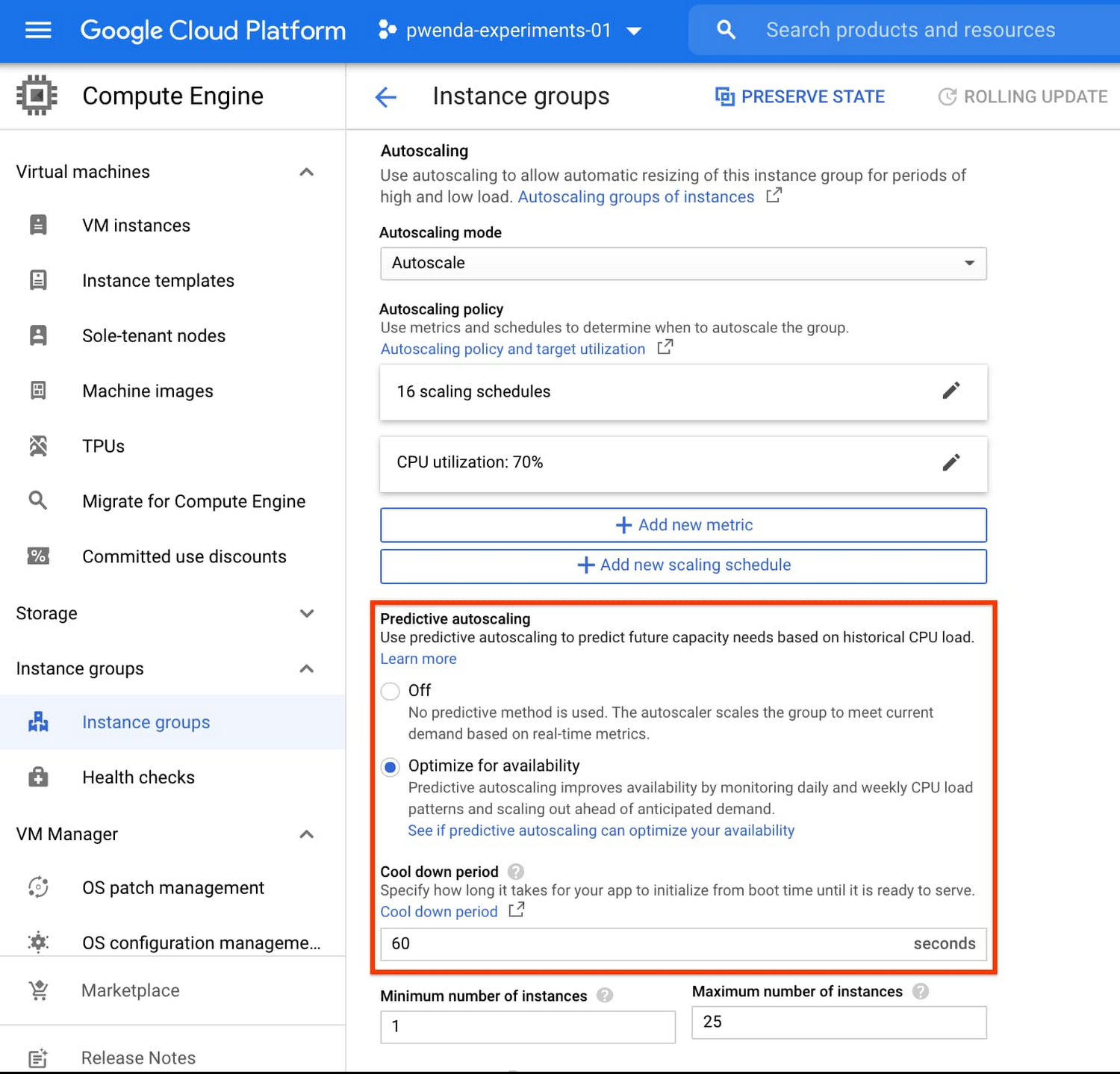
You can enable predictive autoscaling in the Google Cloud Console. Select an autoscaled MIG from the instance groups page and click Edit group. Change predictive autoscaling configuration from Off to Optimize for availability.

To better understand whether predictive autoscaling is good for your application, click the link See if predictive autoscaling can optimize your availability. This will show you a comparison of the last seven days with your current autoscaling configuration vs. with predictive autoscaling enabled.

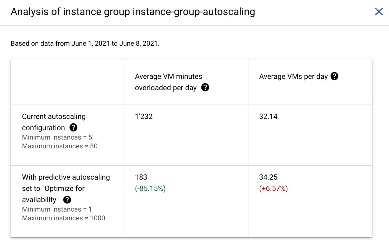
In the above chart, 

• Average VM minutes overloaded per day shows how often your VMs exceed your CPU utilization target. This happens when demand is higher than available capacity. Predictive autoscaling can reduce this by starting VMs ahead of anticipated load. 
• Average VMs per day is a proxy for cost. This shows how much additional VM capacity you need to keep your CPU utilization within the target you have set. You can optimize your cost by adjusting Minimum instances andCPU utilization as explained below. 

Optimizing your configuration

Make sure your Cool down period reflects how long it takes for your application to initialize from VM boot time until it’s ready to serve the load. Predictive autoscaling will use this value to start VMs ahead of forecasted load. If you set it to 10 minutes (600 seconds) your VMs will start 10 minutes before the load is expected to increase.

Review your autoscaling CPU utilization target and Minimum number of instances. With predictive autoscaling you no longer need a buffer to compensate for the time it takes for a VM to start. If your application works best at 70% CPU utilization you don’t need to set target to a much lower value as predictive autoscaling will start VMs ahead of usual load. A higher CPU utilization and lower Minimum number of instances allows you to reduce the cost as you don’t need to pay for additional capacity to prepare for growing demand.

Try predictive autoscaling today

Predictive autoscaling is generally available across all Google Cloud regions. For more information on how to configure, simulate and monitor predictive autoscaling, consult the documentation.

One of India’s best-known healthcare brands, Manipal Group prides itself on clinical excellence and a patient-centric approach. From humble beginnings in 1953 as a single teaching hospital—the Kasturba Medical College—in a university town in Karnataka, India, Manipal Group has grown to a presence in seven cities in India and operations in Malaysia and Nigeria. “Our founder, Dr T. M. A. Pai, established Kasturba Medical College just six years after India gained independence,” says C. G. Muthana, Chief Operating Officer, Teaching Hospitals, Manipal Health Enterprises Pvt. Ltd, part of Manipal Group.

Manipal Health Enterprises Pvt. Ltd operates 11 corporate, or for-profit, hospitals and five teaching hospitals. “We have about 7,000 beds India-wide, and on that measure, we are the third-largest private-sector healthcare provider in India today,” says Muthana. The organization now employs about 6,000 people in its corporate hospitals and 5,000 people in its teaching hospitals.

Manipal Health Enterprises Pvt. Ltd acquires and operates world-class medical technologies in its teaching and corporate hospitals. However, with 75% of corporate hospital wards allocated to fee-paying private patients—compared to just 25% of the wards in teaching hospitals—the differences in information technology budgets are significant. “In the general wards that comprise most of the wards in teaching hospitals, patients are typically treated for free or at heavily subsidized rates,” explains Muthana. “So revenues and costs of delivery vary between hospitals, while employee costs remain similar.”

Rostering nurses a critical task

Rostering nurses to work shifts is one of the most important tasks at Manipal Group corporate and teaching hospitals. As at all hospitals, nurses administer medications, monitor patients, maintain records, manage intravenous lines, and work with doctors to heal patients. They can also provide advice and support to patients and loved ones, including teaching them how to administer medication outside a hospital setting. If too few nurses are rostered for a particular shift, the quality of patient care may suffer.

Google Cloud results

• Enabled the hospital to correctly size its nursing workforce
• Lowers stress on nurses by delivering more equitable rostering
• Presents opportunity to better manage nurses’ leave and other administration tasks

However, rostering at the group’s hospitals was a time-consuming exercise. Senior nurses on each ward would have to spend up to 45 minutes per day manually amending paper-based rosters to accommodate requested changes to duty shifts for personal or other circumstances. The organization began receiving complaints from patients, doctors, and other hospital staff that, on occasion, too few nurses were rostered on for certain shifts—particularly at its flagship hospital in Bangalore. “We had based our rostering calculations on the number of beds occupied by patients and, when we investigated, we found at a macro level, we were rostering on the correct number of nurses,” says Muthana. “However, on some days, on wards optimally staffed by, say, 10 nurses per shift, we might have 14 nurses rostered on for one shift and seven rostered on for another shift. Those times we had seven, we had a clear shortage.”

In 2012, Muthana asked a consultant to develop algorithms to help automate the rostering. “Unfortunately, there were so many variables, the consultant failed to solve the problem,” he says. The Chief Operating Officer’s next step was to ask the founder and Chief Executive Officer of predictive analytics business Retigence Technologies—already working with the business on a materials management project—to develop an application to manage rostering.

Removing the daily drudgery

“Our plan with the automation project was to relieve our senior nurses of the daily drudgery of amending the rosters and to deliver rosters that were as fair as possible to all our staff,” says Muthana. “We also saw an opportunity to reduce our costs by reducing the overall number of nurses needed to look after our patients.”

Retigence Technologies’ team members then worked with the group’s nurses to capture the variables and requirements for the project. For example, a minimum number of nurses with one year experience or more needs to be rostered on for each shift. Retigence Technologies then started building an application using compute resources available through Compute Engine, a Google Cloud product. “We selected Google primarily because of its pioneering work in artificial intelligence (AI) and machine learning,” says Srinibas Behera, founder and Chief Executive Officer of Retigence Technologies.

With the nurses rostering application developed, Manipal Health Enterprises Pvt. Ltd undertook several pilots to build user acceptance. “Some of our senior nurses took time to accept the fact automation removed their control over rostering assignments, but were finally convinced by the better transparency the product offered,” says Muthana. The organization deployed the application to a smaller hospital and secured user support before rolling out the application to its Bangalore flagship.

Eliminating stress

Deploying the application has enabled Manipal Health Enterprises Pvt. Ltd to remove a buffer of about 100 nurses retained to accommodate the variations in number of nurses rostered for individual shifts. “The savings on those salaries more than paid for the cost of developing the application,” says Muthana.

The application also enabled the organization to reduce the stress on nurses—both the nurses in charge of the rosters and the nurses subject to the rosters. “Night shifts were more equitably distributed among the nurses, while we have been able to reduce the 45 minutes per day required to amend rosters to just 10 minutes,” says Muthana. “In Bangalore alone, we have 51 nurses in charge of rostering—so the combined saving there equates to nearly 30 hours per day.” This is freeing up these senior nurses to complete more important tasks.

The application was subsequently implemented at Kasturba Hospital, Manipal, again reducing the time needed to generate complete nursing rosters to less than 10 minutes.

Managing leave and training

The organization now plans to extend the application to manage leave and training for its nurses and other employees. “I would like to see every employee given an annual leave plan that is added to the roster at the start of the year,” says Muthana. “The flexibility and control afforded by the application would enable us to address challenges such as managing leave across a workforce with high attrition rates.” The organization would also be able to create a calendar to ensure nurses receive all their required training.

“We also plan to keep fine-tuning the application to deploy nurses more efficiently and continue to reduce their stress levels,” adds Muthana. “We also want to create a nursing load indicator tailored to patients’ specific circumstances. For example, a sedated patient may not require much nursing care, whereas a patient who comes in with a broken leg and may be on a ventilator may require assistance from three nurses at once.” The business plans to use Google’s AI and machine learning APIs in the future to improve the value and user experience of the product.