





How to Build A Basic Image Search Utility for Natural Language Queries

4704
Of your peers have already read this article.
6:00 Minutes
The most insightful time you'll spend today!
This post shows how to build an image search utility using natural language queries. Our aim is to use different GCP services to demonstrate this. At the core of our project is OpenAI’s CLIP model. It makes use of two encoders – one for images and one for texts. Each encoder is trained to learn representations such that similar images and text embeddings are projected as close as possible.
We will first create a Flask-based REST API capable of handling natural language queries and matching them against relevant images. We will then demonstrate the use of the API through a Flutter-based web and mobile application. Figure 1 shows how our final application would look like:
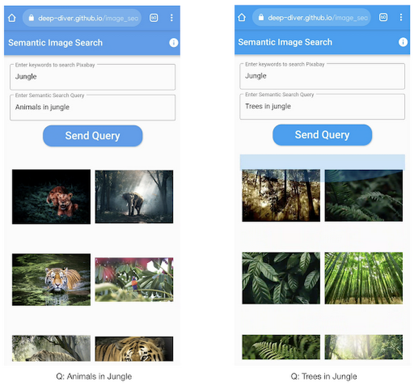
All the code shown in this post is available as a GitHub repository. Let’s dive in.
Application at a high-level
Our application will take two queries from the user:
- Tag or keyword query. This is needed in order to pull a set of images of interest from Pixabay. You can use any other image repositories for this purpose. But we found Pixabay’s API to be easier to work with. We will cache these images to optimize the user experience. Suppose we wanted to find images that are similar to this query: “horses amidst flowers”. For this, we’d first pull in a few “horse” images and then run another utility to find out the images that best match our query.
- Longer or semantic query that we will use to retrieve the images from the pool created in the step above. These images should be semantically similar to this query.
Note: Instead of two queries, we could have only taken a single long query and run named-entity extraction to determine the most likely important keywords to run the initial search with. For this post, we won’t be using this approach.
Figure 2 below depicts the architecture design of our application and the technical stack used for each of the components.
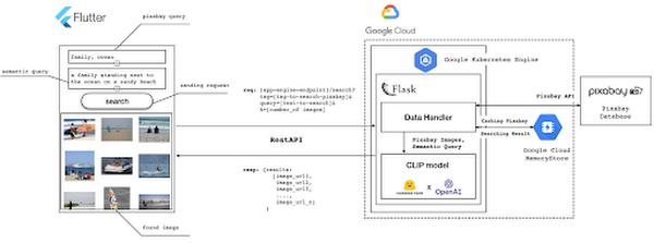
Figure 2 also presents the core logic of the API we will develop in bits and pieces in this post. We will deploy this API on a Kubernetes cluster using the Google Kubernetes Engine (GKE). The following presents a brief directory structure of our application code-base:
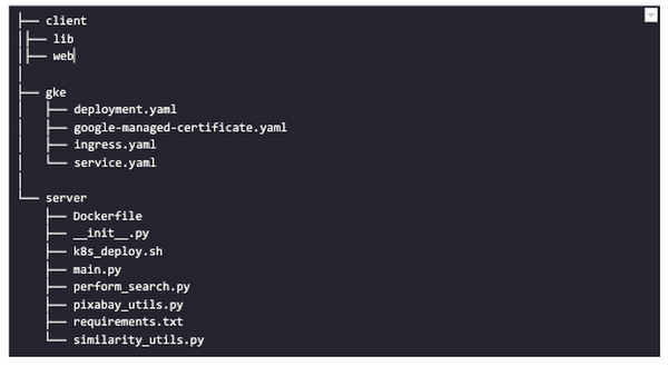
Next, we will walk through the code and other related components for building our image search API. For various machine learning-related utilities, we will be using PyTorch.
Building the backend API with Flask
First, we’d need to fetch a set of images with respect to user-provided tags/keywords before performing the natural language image search. The utility below from the pixabay_utils.py script can do this for us:
def fetch_images_tag(pixabay_search_keyword, num_images):"""Fetches images from Pixabay w.r.t a keyword.:param pixabay_search_keyword: Keyword to perform the search on Pixabay.:param num_images: Number of images to retrieve.:return: List of PIL images.:return: List of image URLs."""query = (PIXABAY_API+ "&q="+ pixabay_search_keyword.lower()+ "&image_type=photo&safesearch=true&per_page="+ str(num_images))response = requests.get(query)output = response.json()all_images = []all_image_urls = []for each in output["hits"]:imageurl = each["webformatURL"]response = requests.get(imageurl)image = Image.open(BytesIO(response.content)).convert("RGB")all_images.append(image)all_image_urls.append(imageurl)return (all_images, all_image_urls)
Note that all the API utilities are logging relevant information. But for brevity, we have omitted the lines of code responsible for that. Next, we will see how to invoke the CLIP model and select the images that would best match a given query semantically. For this, we’ll be using Hugging Face, an easy-to-use Python library offering state-of-the-art NLP capabilities. We’ll collate all the logic related to this search inside a SimilarityUtil class:
class SimilarityUtil:def __init__(self):self.model = CLIPModel.from_pretrained(CLIP_MODEL)self.processor = CLIPProcessor.from_pretrained(CLIP_PREPROCESSOR)self.device = "cuda" if torch.cuda.is_available() else "cpu"def perform_sim_search(self, images, query_phrase, top_k=3):"""Performs similarity search between the images and query.:param images: A list of PIL images initially retrieved withrespect to some entity e.g. Tiger.:param query_phrase: A list containing a single text query,e.g. "Tiger drinking water".:param top_k: Number of top images to return from `images`.:return: Top-k indices matching the query semantically andtheir similarity scores."""model = self.model.to(self.device)# Obtain the text-image similarity scoreswith torch.no_grad():inputs = self.processor(text=[query_phrase], images=images, return_tensors="pt", padding=True)inputs = inputs.to(self.device)outputs = model(**inputs)# Image-text similarity scoreslogits_per_image = outputs.logits_per_image.cpu()(top_indices, top_scores) = self.sort_scores(logits_per_image, top_k)return (top_indices, top_scores)def sort_scores(self, scores, top_k):"""Sorts the scores in a descending manner.:param scores: Scores to sort through.:param top_k: Number of top scores to return.:return: Top-k scores and their indices."""values, indices = scores.squeeze().topk(top_k)top_indices, top_scores = [], []for score, index in zip(values, indices):top_indices.append(int(index.numpy()))score = score.numpy().tolist()top_scores.append(round(score, 3))return (top_indices, top_scores)
CLIP_MODEL uses a ViT-base model to encode the images for generating meaningful embeddings with respect to the provided query. The text-based query is also encoded using A Transformers-based model for generating the embeddings. These two embeddings are matched with one another during inference. To know more about the particular methods we are using for the CLIP model please refer to this documentation from Hugging Face.
In the code above, we are first invoking the CLIP model with images and the natural language query. This gives us a vector (logits_per_image) that contains the similarity scores between each of the images and the query. We then sort the vector in a descending manner. Note that we are initializing the CLIP model while instantiating the SimilarityUtil to save us the model loading time. This is the meat of our application and we have tackled it already. If you want to interact with this utility in a live manner you can check out this Colab Notebook.
Now, we need to collate our utilities for fetching images from Pixabay and for performing the natural language image search inside a single script – perform_search.py. Following is the main class of that script:
class Searcher:def __init__(self):self.similarity_model = SimilarityUtil()def get_similar_images(self, keyword, semantic_query, pixabay_max, top_k):"""Finds semantically similar images.:param keyword: Keyword to search with on Pixabay.:param semantic_query: Query to find semantically similar images retrieved from Pixabay.:param pixabay_max: Number of maximum images to retrieve from Pixabay.:param top_k: Top-k images to return.:return: Tuple of top_k URLs and the similarity scores of the images present inside the URLs."""images_redis_key = keyword + "_images"urls_redis_key = keyword + "_urls"if redis_client.exists(images_redis_key) and redis_client.exists(urls_redis_key):keyword_images = redis_client.get(images_redis_key)keyword_image_urls = redis_client.get(urls_redis_key)else:(keyword_images, keyword_image_urls) = fetch_images_tag(keyword, pixabay_max)redis_client.set(images_redis_key, keyword_images)redis_client.set(urls_redis_key, keyword_image_urls)(top_indices, top_scores) = self.similarity_model.perform_sim_search(keyword_images, semantic_query, top_k)top_urls = [keyword_image_urls[index] for index in top_indices]return (top_urls, top_scores)
Here, we are just calling the utilities we had previously developed to return the URLs of the most similar images and their scores. What is even more important here is the caching capability. For that, we combined GCP’s MemoryStore and a Python library called direct-redis. More on setting up MemoryStore later.
MemoryStore provides a fully managed and low-cost platform for hosting Redis instances. Redis databases are in memory and light-weight making them an ideal candidate for caching. In the code above, we are caching the images fetched from Pixabay and their URLs. So, in the event of a cache hit, we won’t need to call the CLIP model and this will tremendously improve the response time of our API.
Other options for caching
We can cache other elements of our application. For example, the natural language query. When searching through the cached entries to determine if it’s a cache hit, we can compare two queries for semantic similarity and return results accordingly.
Consider that a user had entered the following natural language query: “mountains with dark skies”. After performing the search, we’d cache the embeddings of this query. Now, consider that another user entered another query: “mountains with gloomy ambiance”. We’d compute its embeddings and run a similarity search with the cached embeddings. We’d then compare the similarity scores with respect to a threshold and parse the most similar queries and their corresponding results. In case of a cache miss, we’d just call the image search utilities we developed above.
When working on real-time applications we often need to consider these different aspects and decide what enhances the user experience and maximizes business at the same time.
All that’s left now for the backend is our Flask application – main.py:
@app.route("/search", methods=["GET"])def get_images():tag = request.args.get("t").lower()query = request.args.get("s_query").lower()top_k = request.args.get("k")(top_urls, top_scores) = searcher.get_similar_images(tag, query, MAX_PIXABAY_SEARCH, int(top_k))return jsonify({"top_urls": top_urls, "top_scores": top_scores})
Here we are first parsing the query parameters from the request payload of our search API. We are then just calling the appropriate function from perform_search.py to handle the request. This Flask application is also capable of handling CORS. We do this via the flask_cors library:
cors = CORS(app,resources={r"/search/*": {"origin": "*"},r"/test/*": {"origin": "*"},},)
And this is it! Our API is now ready for deployment.
Deployment with Compute Engine and GKE
The reason why we wanted to deploy our API on Kubernetes is because of the flexibility Kubernetes offers for managing deployments. When operating at scale, auto scalability and load balancing are very important. With the comes the requirement of security — we’d not want to expose the utilities for interacting with any internal services such as databases. With Kubernetes, we can achieve all these easily and efficiently.
GKE provides secured and fully managed functionalities for operationalizing Kubernetes clusters. Here are the steps to deploy the API on GKE at a glance:
- We first build a Docker image for our API and then push it to the Google Container Registry (GCR).
- We then create a Kubernetes cluster on GKE and initialize a deployment.
- We then add scalability options.
- If any public exposure is needed for the API, we then tackle it.
We can assimilate all the above into a shell script – k8s_deploy.sh:
## Docker build and push ### We are inside the `server` directorydocker build -t gcr.io/${PROJECT_ID}/search_service .docker push gcr.io/${PROJECT_ID}/search_service## Deploy on a GKE cluster ### Configure the Docker command-line tool to authenticate to Container Registrygcloud auth configure-docker# Create a Kubernetes clustergcloud container clusters create image-search-nlp# Create a deploymentkubectl create deployment clip-search --image=gcr.io/${PROJECT_ID}/search_service# Number of worker replicaskubectl scale deployment clip-search --replicas=3# HorizontalPodAutoscaler resourcekubectl autoscale deployment clip-search --cpu-percent=80 --min=1 --max=5# Expose deploymentkubectl expose deployment clip-search --name=clip-search-service --type=LoadBalancer --port 80 --target-port 8080
These steps are well explained in this tutorial that you might want to refer to for more details. We can configure all the dependencies on our local machine and execute the shell script above. We can also use the GCP Console to execute it since a terminal on the GCP Console is pre-configured with the system-level dependencies we’d need. In reality, the Kubernetes cluster should only be created once and different deployment versions should be created under it.
After the above shell script is run successfully, we can run kubectl get service to know the external IP address of the service we just deployed:
NAME CLUSTER-IP EXTERNAL-IP PORT(S) AGEclip-search-service 10.3.251.122 203.0.113.0 80:30877/TCP 10s
We can now consume this API with the following base URI: http://203.0.113.0/. If we wanted to deal with only http-based API requests, then we are done here. But secured communication is often a requirement in order for applications to operate reliably. In the following section, we are to discuss how to configure the additional items to allow our Kubernetes cluster to allow https requests.
Configurations for handling https requests with GKE
A secure connection is almost often a must-have requirement in modern client/server applications. The front-end Flutter application would be hosted on GitHub Pages for this project, and it requires https-based connection as well. Even if configuring https connection particularly for a GKE-based cluster can be considered a chore, its setup might seem daunting at first.
There are six steps to configure https connection in the GKE environment:
- You need to have a domain name, and there are a lot of inexpensive options that you can buy. For instance, mlgde.com domain for this project is acquired via Gabia which is a Korean service provider.
- A reserved (static) external IP address has to be acquired via gcloud command or GCP console.
- You need to bind the domain name with the acquired external IP address. This is a platform-specific configuration that issued the domain name to you.
- There is a special ManagedCertificate resource which is specific to the GKE environment. ManagedCertificate resource specifies the domain that the SSL certificate will be created for, so you need this.
- An Ingress resource should be created by listing the static external IP address, ManagedCertificate resource, and the service name and port which the incoming traffic will be routed to. The Service resource could remain the same as in the above section with only changes from LoadBalancer to ClusterIP.
- Last but not least, you need to modify the existing Flask application and Deployment resource to support liveness and readiness probes which are used to check the health status of the Deployment. The Flask application side can be simply modified with the flask-healthz Python package, and you only need to add
livenessProbeandreadinessProbesections in the Deployment resource. In the code example below, thelivenessProbeandreadinessProbeare checked via/aliveand/readyendpoints respectively.
from flask_healthz import healthzfrom flask_healthz import HealthErrorapp = Flask(__name__)app.register_blueprint(healthz, url_prefix="/")def printok():print("Everything is fine")def liveness():try:printok()except Exception:raise HealthError("Can't connect to the file")def readiness():try:printok()except Exception:raise HealthError("Can't connect to the file")app.config.update(HEALTHZ = {"alive": "main.liveness","ready": "main.readiness",})
One thing to be careful of is the initialDelaySeconds attribute of the probes. It is uncommon to configure this attribute with a big number, but it could be bigger than 90 – 120 seconds depending on the size of the model to be used. For this project, it is configured in 90 seconds in order to wait until the CLIP model is fully loaded into memory (full YAML script here).
livenessProbe:httpGet:path: /aliveport: 8080initialDelaySeconds: 90periodSeconds: 10readinessProbe:httpGet:path: /readyport: 8080initialDelaySeconds: 90periodSeconds: 10
Again, these steps may seem daunting at first, but it will become clear when you have done it once. Here is the official document for Using Google-managed SSL certificates You can find all the GKE-related resources used in this project here.
Once every step is completed you should be able to see your server application running on the GKE environment. Please make sure to run kubectl apply command whenever you create Kubernetes resources such as Deployment, Service, Ingress, and ManagedCertificate, and it is important to wait for more than 10 minutes until the ManagedCertifcate provisioning is done.
You can run gcloud compute addresses list command to find out the static external IP address that you have configured.
NAME ADDRESS/RANGE TYPE PURPOSE NETWORK REGION SUBNET STATUSgde 34.149.231.34 EXTERNAL IN_USE
Then, the IP address has to be mapped to the domain. Figure 3 is a screenshot of a dashboard from where we got the mlgde.com domain. It clearly shows mlgde.com is mapped to the static external IP address configured in GCP.
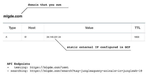
In case you’re wondering why we didn’t deploy this application on App Engine, well that is because of the compute needed to execute the CLIP model. App Engine instance won’t fit in that regime. We could have also incorporated compute-heavy capabilities via a VPC Connector. That is a design choice that you and your team would need to consider. In our experiments, we found the GKE deployment to be easier and suitable for our needs.
Infrastructure for the CLIP model
As mentioned earlier, at the core of our application is the CLIP model. It is computationally a bit more expensive than the regular deep learning models. This is why it makes sense to have the hardware infrastructure set up accordingly to execute it. We ran a small benchmark in order to see how a GPU-based environment could be beneficial here.
We ran the CLIP on a Tesla P100-based machine and also on a standard CPU-only machine 1000 times. The code snippet below is the meat of what we executed:
DEVICE = "cuda" if torch.cuda.is_available() else "cpu"start_time = time.time()for _ in range(1000):with torch.no_grad():model = model.to(DEVICE)inputs = processor(text=[semantic_search_phrase],images=all_images, return_tensors="pt", padding=True)inputs = inputs.to(DEVICE)outputs = model(**inputs)end_time = time.time() - start_timeprint(f"Total time: {end_time:.3f} seconds.")
As somewhat expected, with the GPU, the code took 13 minutes to complete execution. With no GPU, it took about 157 minutes.
It is uncommon to leverage GPUs for model prediction because of cost restrictions, but sometimes we have to access GPUs for deploying a big model like CLIP. We configured a GPU-based cluster on GKE and compared the performance differences with and without it. It took about 1 second to handle a request with GPU and MemoryStore cache while it took more than 4 seconds with MemoryStore only (without the GPUs).
For the purposes of this post, we used a CPU-based cluster on Kubernetes. But It is easy to configure GPU usage in a GKE cluster. This document shows you how to do so. For a short summary, there are two steps. First, a node should be configured with GPUs when creating a GKE cluster. Second, GPU drivers should be installed in GKE nodes. You don’t need to visit and manually install GPU drivers for each node by yourself. Rather you can simply apply the DaemonSet resource to GKE as described here.
Setting up MemoryStore
In this project, we first query the general concept of images to Pixabay, then we filter the images with a semantic query using CLIP. It means we can cache the initially retrieved images from Pixabay for the next specific semantic query. For instance, you may want to search with “gentleman wearing tie” at first, then you may want to retry searching for “gentleman wearing glass”. In this case, the base images remain all the same, so they could be stored in a cache server like Redis.
MemoryStore is a GCP service wrapping the Redis which is an in-memory data store, so you can simply use a standard Redis Python package for accessing it. The only thing to be careful about when provisioning a MemoryStore Redis instance is to make sure it is in the same region where your GKE cluster or Compute Engine instance is.
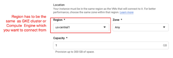
The code snippet below shows how to make a connection to the Redis instance in Python. Nothing specific to GCP, but you only need to be aware of the usage of the standard redis-py package.
# REDISHOST is the IP address to the MemoryStore instanceredis_host = os.environ.get("REDISHOST", "localhost")redis_port = int(os.environ.get("REDISPORT", 6379))redis_client = redis.StrictRedis(host=redis_host, port=redis_port)
After creating a connection, you can store and retrieve data from MemoryStore. There are more advanced use cases of Redis, but we only used exists, get, and set methods for the demonstration purpose. These methods should be very familiar if you know maps, dictionaries, or other similar data structures. For the code portion that uses Redis-related utilities, please refer to the Searcher Python class we discussed in an earlier section.
In the URLs below, you can find side-by-side comparisons of using MemoryStore:
- Without MemoryStore: https://youtu.be/7B88Eyrd-4s
- With MemoryStore (1st try): https://youtu.be/LE6xeEIRuMM
- With MemoryStore (2nd try): https://youtu.be/rRfK17sdk84
Putting everything together
All that’s left now is to collate the different components we developed in the sections above and deploy our application with a frontend. All the frontend-related code is present here.
- The front-end application is written in the Flutter development kit. The main screen contains two text fields for queries to Pixabay and CLIP model respectively. When you click the “Send Query” button, it will send out a RestAPI request to the server. After receiving the result back from the server, the retrieved images from the semantic query will be displayed at the bottom section of the screen.
- Please note that a Flutter application can be deployed to various environments including desktop, web, iOS, and Android. In order to keep as simple as possible, we chose to deploy the application to the GitHub Pages. Whenever there is any change to a client-side source directory, the GitHub Action will be triggered to build a web page and deploy the latest version to the GitHub Pages.
Our final application is deployed here and it looks like so:
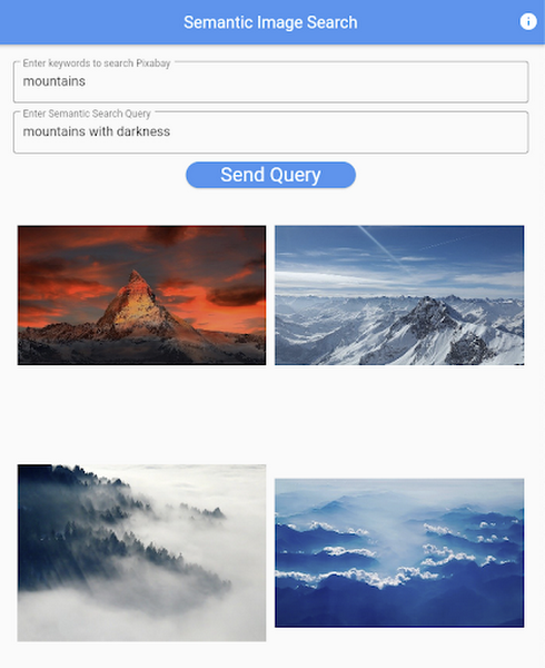
Note that due to constraints, the above-mentioned URL will only be live for one or two months.
It is also possible to redeploy the back-end application with a GitHub Action.
- The very first step is to craft a Dockerfile like below. Since Python is a scripting language, and there are lots of heavy packages that the application is dependent on, it is important to cache the steps. For instance, installing the dependencies should be separated from other commands.
FROM pytorch/pytorch:latestWORKDIR /app# install the dependenciesCOPY requirements.txt requirements.txtRUN pip install -r requirements.txtCOPY . .# set up environment variablesENV PIXABAY_API_KEY="..."ENV REDIS_IN_USE="true"ENV REDISHOST="..."# expose port that Flask app is listening onEXPOSE 8080# run the Flask appCMD [ "python3", "main.py" ]
- With the Dockerfile defined, we can use a GitHub Action like this for automatic deployment.
Edge cases
Since the CLIP model is pre-trained on a large corpus of image and text pairs it’s likely that it may not generalize well to every natural language query we throw at it. Also, because we are limiting the number of images on which the CLIP model can operate, this somehow restricts the expressivity of the model.
We may be able to improve the performance for the second situation by increasing the number of images to be pre-fetched and by indexing them into a low-cost and high-performance database like Datastore.
Costs
In this section, we wanted to provide the readers a breakdown of the costs they might incur in order to consume the various services used throughout the application.
- Frontend hosting
- The front-end application is hosted on GitHub Pages, so there is no expenditure for this.
- Compute Engine
- With an e2-standard-2 instance type without GPUs, the cost is around $48.92 per month. In case you want to add a GPU (NVIDIA K80), the cost goes up to $229.95 per month.
- MemoryStore
- The cost for MemoryStore depends on the size. With 1GB of space, the cost is around $35.77 per month, and whenever you add more GBs the cost will be doubled.
- Google Kubernetes Engine
- The monthly cost for a 3 node GKE cluster with n2-standard-2 (vCPUs: 2, RAM: 8GB without GPUs) is about $170.19. If you add one GPU (NVIDIA K80) to the cluster, the cost goes up to $835.48.
While you may think that is a lot cost-wise, it is good to know that Google gives away free $300 credits when you create a new GCP account. It is still not enough for leveraging GPUs, but it is enough to learn and experiment with GKE and MemoryStore usage.
Conclusion
In this post, we walked through the components needed to build a basic image search utility for natural language queries. We discussed how these different components are connected to each other. Our image search API is able to utilize caching and was deployed on a Kubernetes cluster using GKE. These elements are essential when building a similar service to cater to a much bigger workload. We hope this post will serve as a good starting point for that purpose. Below are some references on similar areas of work that you can explore:
- Building a real-time embeddings similarity matching system
- Detecting image similarity using Spark, LSH and TensorFlow
Acknowledgments: We are grateful to the Google Developers Experts program for supporting us with GCP credits. Thanks to Karl Weinmeister and Soonson Kwon of Google for reviewing the initial draft of this post.
How Vertex Vizier’s Automated Hyperparameter Tuning Improves ML Models

5050
Of your peers have already read this article.
1:30 Minutes
The most insightful time you'll spend today!
We recently launched Vertex AI to help you move machine learning (ML) from experimentation into production faster and manage your models with confidence—speeding up your ability to improve outcomes at your organization.
But we know many of you are just getting started with ML and there’s a lot to learn! In tandem with building the Vertex AI platform, our teams are dropping as much best practices content as we can to help you come up to speed. Plus, we have a dedicated event on June 10th, Applied ML Summit, with sessions on how to apply ML technology in your projects, as well as grow your skills in this field.
In the meantime, we couldn’t resist a quick lesson on hyperparameter tuning, because (a) it’s incredibly cool (b) you will impress your coworkers (c) Google Cloud has some unique battle tested tech in this area and (d) you will save time by getting better ML models into production faster. Vertex Vizier, on average, finds optimal parameters for complex functions in over 80% fewer trials than traditional methods.
So it’s incredibly cool, but what is it?
While machine learning models automatically learn from data, they still require user-defined knobs which guide the learning process. These knobs, commonly known as hyperparameters, control, for example, the tradeoff between training accuracy and generalizability. Examples of hyperparameters are the optimizer being used, its learning rate, regularization parameters, the number of hidden layers in a DNN, and their sizes.
Setting hyperparameters to their optimal values for a given dataset can make a huge difference in model quality. Typically, optimal hyperparameter values are found via grid searching a small number of combinations, or tedious manual experimentation. Hyperparameter tuning automates this work for you by searching for the best configuration of hyperparameters for optimal model performance.
Vertex Vizier enables automated hyperparameter tuning in several ways:
- “Traditional” hyperparameter tuning: by this we mean finding the optimal value of hyperparameters by measuring a single objective metric which is the output of an ML model. For example, Vizier selects the number of hidden layers and their sizes, an optimizer and its learning rate, with the goal of maximizing model accuracy.
- When hyperparameters are evaluated, models are trained and evaluated on splits of the data set. If evaluation metrics are streamed to Vizier (e.g. as a function of epoch) as the model is trained, Vizier’s early stopping algorithms can predict the final objective value, and recommend which unpromising trials should be early stopped. This conserves compute resources and speeds up convergence.
- Oftentimes, models are tuned sequentially on different data sets. Vizier’s built in transfer learning learns priors from previous hyperparameter tuning studies, and leverages them to converge faster on subsequent hyperparameter tuning studies.
- AutoML is a variant of #1, where Vertex Vizier performs both model selection, and also tunes architectures/non-architecture modifying hyperparameters. AutoML usually requires more code on top of Vertex Vizier (to ingest data etc), but Vizier is in most cases the “engine” behind the process. AutoML is implemented by defining a tree like (DAG) search space, rather than a “flat” search space (like in #1). Note that you can use DAG search spaces for any other purpose where searching over a hierarchical space makes sense.
- There are times when you may wish to optimize more than one metric. For example, we would like to optimize model accuracy, while minimizing model latency. Vizier can find the Pareto frontier, which presents tradeoffs for multiple metrics, allowing users to choose the appropriate tradeoff. Simple example: I want to make a more accurate model, but would like to minimize serving latency. I do not know ahead of time what’s the tradeoff between the two metrics. Vizier can be used to explore and plot a tradeoff curve, so users can select on the most appropriate one. For example, “a latency decrease of 200ms will only decrease accuracy by 0.5%”
Google Vizier is all yours with Vertex AI
Google published the Vizier research paper in 2017, sharing our work and use cases for black-box optimization—i.e. The process of finding the best settings for a bunch of parameters or knobs when you can’t peer inside a system to see how well the knobs are working. The paper discusses our requirements, infrastructure design, underlying algorithms, and advanced features such as transfer learning that the service provides. Vizier has been essential to our progress with machine learning at Google, which is why we are so excited to make it available to you on Vertex AI.
Vizier has already tuned millions of ML models at Google, and its algorithms are continuously improved for faster convergence and handling of real-life edge cases. Vertex Vizier’s models are very well calibrated and are self-tuning (they adapt to user data), and offer unique power features, such as hierarchical search spaces and multi-objective optimization. We believe Vertex Vizier’s set of features is a unique capability to Google Cloud, and look forward to optimizing the quality of your models by automatically tuning hyperparameters for you.
To learn more about Vertex Vizier, check out these docs and if you are interested in what’s coming in machine learning over the next five years, tune in to our Applied ML Summit on June 10th, or watch the sessions on demand in your own time.
3158
Of your peers have already watched this video.
2:00 Minutes
The most insightful time you'll spend today!
How Marketers Can Turn Information into Action with Machine Learning
The biggest challenge marketers face with machine learning is, “how to get starter”? Instead of getting overwhelmed, they should focus on the applied machine learning by using the algorithms that are already built.
Cassie Kozyrkov, the chief decision scientist with Google Cloud, says that marketers who are overwhelmed by everything they’re hearing about machine learning should focus on key ingredients, not building an entire kitchen.
Increasing Production Efficiency: How AI Can Improve Asset Utilization and Minimize Downtime

2703
Of your peers have already read this article.
1:30 Minutes
The most insightful time you'll spend today!
Today, manufacturers are advancing on their factory digitalization journey, betting on innovative technologies to strengthen competitiveness, deliver sustainable growth, and offer new services. Macroeconomic factors – such as high energy costs, increasing labor, and raw material shortages – drive the need for urgent operational optimizations and automation.
Cloud capabilities have matured at an accelerated pace, giving manufacturers practical avenues to achieve these goals. Manufacturers are finding new ways to bring AI and machine learning (ML) to practical use cases, like predictive maintenance, anomaly detection, and asset utilization management. However, manufacturers struggle to adopt AI at scale due to challenges around data accessibility, infrastructure, and technology.
Google Cloud created purpose-built tools and solutions to organize manufacturing data, make it accessible and useful, and help manufacturers quickly take significant steps on this journey by reducing the time to value. In this post, we will explore a practical example of how manufacturers can use Google Cloud manufacturing solutions to train, deploy and extract value from ML-enabled capabilities to predict asset utilization and maintenance needs.
The journey to machine learning insights starts with accessible data
The first step to a successful machine learning project is to unify necessary data in a common repository. For this, we will use Manufacturing Connect, the factory edge platform co-developed with Litmus Automation, to connect to manufacturing assets and stream the asset telemetries to Pub/Sub.
After the telemetry messages are published to Pub/Sub, Dataflow will identify each message based on its structure and apply corresponding normalizations and transformations, which are preconfigured in Manufacturing Data Engine. Once the messages are processed, the messages will be routed to Cloud Storage, BigQuery, and/or Cloud BigTable based on user configuration.
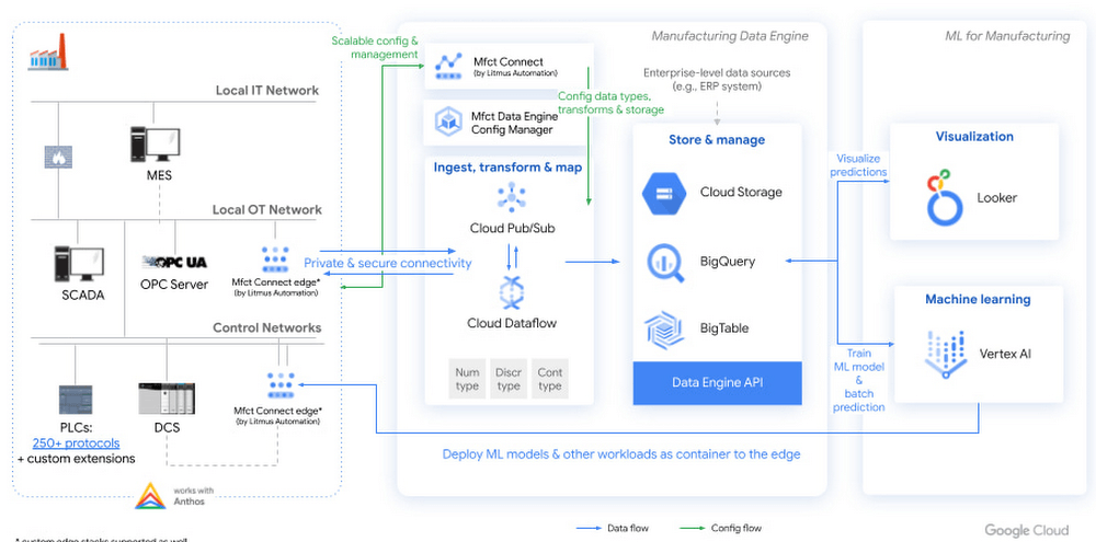
Figure 1. High level architecture diagram of machine learning with Manufacturing Data Engine
To train a machine learning model, manufacturers can use Vertex AI AutoML to build a no-code model based on the training data stored in the Manufacturing Data Engine.
Then, users can trigger a batch prediction job in Vertex AI or export the AutoML model to run on the edge component of Manufacturing Connect for real-time prediction. Regardless of the model deployment methods, the prediction and explanation results will be ingested into Manufacturing Data Engine, which can be analyzed and visualized in Looker.
A blueprint for classifying asset condition
The following scenario is based on a hypothetical company, Cymbal Materials. This company is a factitious discrete manufacturing company that runs 50+ factories in 10+ countries. 90% of Cymbal Materials manufacturing processes involve milling, which are accomplished using industrial computer numerical control (CNC) milling machines. Although their factories implement routine maintenance checklists, there are unplanned and unknown failures that happen occasionally. However, many of the Cymbal Materials factory workers lack the experience to identify and troubleshoot failures due to labor shortage and high turnover rate in their factories. Hence, Cymbal Materials is working with Google Cloud to build a machine learning model that can identify and analyze failures on top of Manufacturing Connect, Manufacturing Data Engine, and Vertex AI.
For the pilot, Cymbal Materials forms a team of manufacturing engineers and data scientists to evaluate the feasibility of solving the tool wear detection problem. To avoid compliance concern, the Cymbal Materials team chooses to start with a public tool wear detection dataset hosted on Kaggle. This dataset is collected from running machining experiments on 2″ x 2″ x 1.5″ wax blocks in a CNC milling machine. The dataset contains measurements from the 4 motors (X,Y, Z axes and spindle) and program values in the CNC machine, which maps well to the data that Cymbal Materials collects for their CNC milling machines.
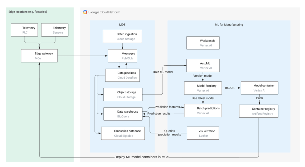
To start, the Cymbal Materials data scientists download the tool wear detection dataset from Kaggle and upload the dataset to Cloud Storage. Then, the data scientists use Vertex AI to:
- Perform exploratory data analysis using Vertex AI Workbench
- Train machine learning models using Vertex AI AutoML
- Deploy machine learning models to perform batch prediction and export AutoML models for edge deployment
- Interpret predictions using Vertex Explainable AI
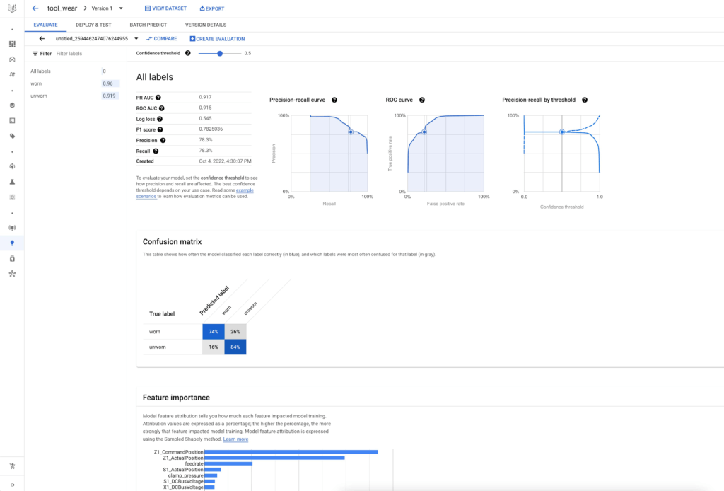
After seeing great performance of the AutoML tabular model, the Cymbal Materials data scientists decide to use the AutoML model to predict on the actual CNC milling machine telemetries from their factories and validate the generalizability of the AutoML model. They ask the manufacturing engineers to deploy Manufacturing Connect in a Cymbal Materials factory and stream telemetries for one CNC milling machine to the Manufacturing Data Engine.
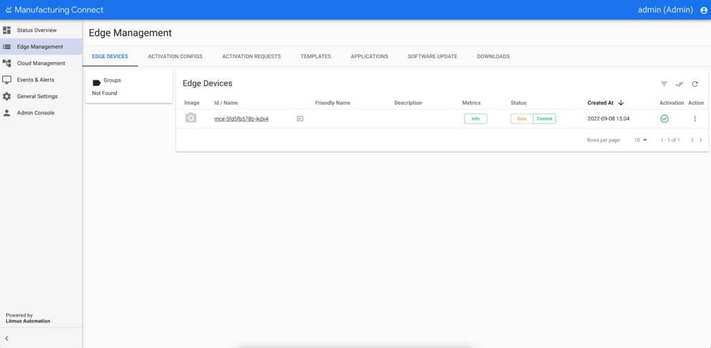
Manufacturing Connect includes an edge component that can gather data from manufacturing assets via an extensive library of 250+ communication protocols. The edge component of Manufacturing Connect comes with built-in Node-RED and Docker runtime, which support running custom workflows and machine learning models at the edge.
Using pre-defined hierarchies, Manufacturing Connect pushes asset telemetries and states to Pub/Sub.
After the factory operational data are ingested into Pub/Sub, Cymbal Materials uses Manufacturing Data Engine to:
- Normalize, transform, and contextualize real-time operational data with slowly changing metadata
- Batch ingest historical operational data and prediction results
- Route data dynamically to Cloud Storage, BigQuery, and/or Cloud BigTable
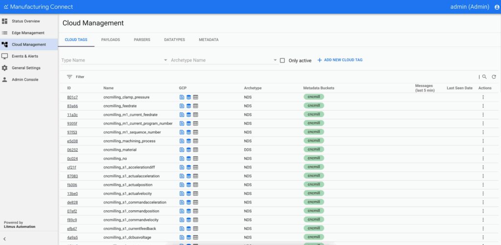
Figure 5. Manufacturing Data Engine configuration in Manufacturing Connect.
Using the trained AutoML tabular model and real-time telemetries from CNC milling machines, the data scientists trigger a batch prediction job on the CNC milling machine telemetries in BigQuery. The data scientists configure the batch prediction to output prediction results in Cloud Storage such that Manufacturing Data Engine can batch ingest the prediction results after the batch prediction job completes.
To consume the prediction results, the Cymbal Materials manufacturing engineers use Looker to create visualizations. The dashboard allows the manufacturing engineers to:
- Visualize the CNC milling machine actual and predicted tool conditions over time
- Explain the prediction results by summarizing the top attributing features
- Create alerts based on the predicted tool condition for their assets
- Take actions by contacting the supplier and/or scheduling maintenance for their assets
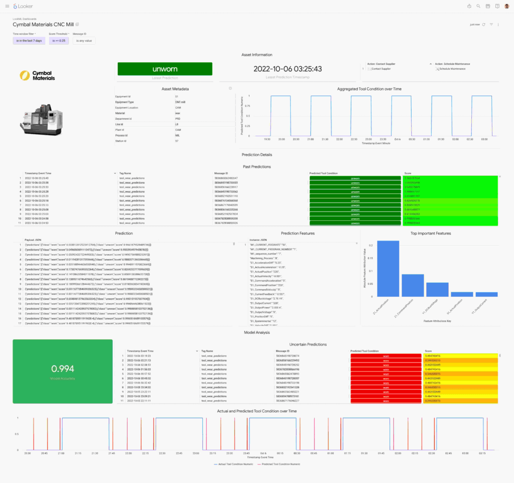
Figure 6. CNC mill wear prediction displayed in a Looker dashboard.
From edge to cloud, improving production efficiency for manufacturers
To support the entire factory digitalization value journey, manufacturers are looking for capabilities from simple visualizations to predictive ML models. Robust solutions, such as the one covered here, provide rapid paths for engineers to extract insight from their factory data.
Having a common data repository for manufacturing data, industry-leading machine learning platform, and versatile dashboard components accelerate manufacturer’s digital transformation.
This solution brings the best of Google Cloud’s data analytics and artificial intelligence capabilities in an industrial environment. Manufacturing Connect creates the link between industrial machinery and Manufacturing Data Engine, the cloud platform where the manufacturing data are processed, normalized, contextualized, and stored in a ready-to-consume format. Vertex AI can build, deploy, and scale machine learning models using data stored in the Manufacturing Data Engine. Vertex AI includes AutoML and Workbench for training models without code and training custom models with code-first experience respectively.
Learn more about how Google Cloud is transforming manufacturing to meet changing customer expectations at our Google Cloud Next Manufacturing playlist.
What’s next
Google’s Latest ‘Carbon Footprint’ can Flag Users about Carbon Emission Levels from their Cloud Usage

7098
Of your peers have already read this article.
4:00 Minutes
The most insightful time you'll spend today!
Google Cloud is proud to support our customers with the cleanest cloud in the industry. For the past four years, we’ve matched 100% of our electricity use with renewable energy purchases, and we were the first company of our size to commit going even further by running on carbon-free energy 24/7 by 2030. As we work to achieve 24/7 carbon-free energy, we help you take immediate action to decarbonize your digital applications and infrastructure. We’re also working with our customers across every industry to develop new solutions for the unique climate change challenges that organizations face. Today, we’re excited to expand our portfolio of carbon-free solutions and announce new partnerships that will help every company build a more sustainable future.
First, we’re launching Carbon Footprint, a new product that provides customers with the gross carbon emissions associated with their Google Cloud Platform usage. Now available to every GCP user for free in the Cloud Console, this tool helps you measure, track and report on the gross carbon emissions associated with the electricity of your cloud usage. Of course, the net operational emissions associated with your Google Cloud usage is still zero. With growing requirements for Environmental Social and Governance (ESG) reporting, companies are looking for ways to show their employees, boards and customers their progress against climate targets. Using Carbon Footprint, you have access to the gross energy related emissions data you need for internal carbon inventories and external carbon disclosures, with one click.
Built in collaboration with customers like Atos, Etsy, HSBC, L’Oréal, Salesforce, Thoughtworks and Twitter, our Carbon Footprint reporting introduces a new standard of transparency to support you in meeting your climate goals. You can monitor your gross cloud emissions over time, by project, by product and by region, giving IT teams and developers metrics that can help them reduce their carbon footprint. Our detailed calculation methodology is published so that auditors and reporting teams can verify that their cloud emissions data meets GHG Protocol guidance.

“The power of knowledge combined with the power of technology innovation plays a vital role in proactively responding to the climate crisis we are facing. With Google Carbon Footprint reporting, Atos feeds emissions data in our Decarbonization Data Platform, demonstrating potential emissions reductions from the Google Cloud Platform to our customers. This reporting opens up new levels of emissions transparency, trajectory planning, and data insight to support our customers in meeting, and potentially accelerating towards, their climate goals.”—Nourdine Bihmane, Head of Decarbonization Business Line, Atos
“The capability to measure and understand the environmental footprint of our Public Cloud usage is among the key axis of our sustainable tech roadmap. With Google Cloud Carbon Footprint, we are now able to directly follow the impact of our sustainable infrastructure approach and architecture principles.”—Hervé DUMAS, Sustainability IT Director, L’Oreal
While digital infrastructure emissions are just one part of your environmental footprint, accurately accounting for IT carbon emissions is necessary to measure progress against the carbon reduction targets required to avert the worst consequences of climate change. To help you account for emissions beyond our cloud and across your organization, we’re excited to partner with Salesforce Sustainability Cloud, integrating our Google Cloud Platform emissions data into their carbon accounting platform.
“As we face unprecedented climate challenges, companies across the globe need to embed sustainability into the core of their business in order to meet growing customer and stakeholder expectations, and reduce their environmental impact. Together, Google Cloud and Salesforce Sustainability Cloud can help our joint customers accelerate their path to Net Zero, leveraging data-driven insights and visualizations to track and reduce their carbon emissions to drive sustainable change.”—Ari Alexander, GM of Salesforce Sustainability Cloud.
From information to action
With the gross energy-related emissions footprint of data associated with your Google Cloud usage now available, we’re committed to providing tools to not only measure your carbon footprint, but help you reduce it. We recently launched low-carbon region icons to help you choose cleaner regions to locate your Google Cloud resources. New users who see the icons are over 50% more likely to choose clean regions over others, ensuring their applications emit less carbon over time.
For current Google Cloud users, we’re pleased to announce that Active Assist Recommender will include a new sustainability impact category, extending its original core pillars of cost, performance, security, and manageability. Starting with the Unattended Project Recommender, you’ll soon be able to estimate the gross carbon emissions you’ll save by removing your idle resources. Unattended Project Recommender uses machine learning to identify, with a high degree of confidence, projects that are likely abandoned based on API and networking activity, billing, usage of cloud services, and other signals, and provides actionable recommendations on how to remediate those abandoned projects. By deleting these projects, not only can you reduce costs and mitigate security risks, but you can also reduce your carbon emissions. In August, Active Assist analyzed the aggregate data from all customers across our platform, and over 600,000 gross kgCo2e was associated with projects that it recommended for cleanup or reclamation. If customers deleted these projects they would significantly reduce future gross carbon emissions. Check out this blog to learn more about Active Assist.

Solutions for climate resilience
Many of our customers face difficult questions about how their business impacts the natural environment today, and how it will be affected by climate change in the future. Answering these questions requires rich datasets about the planet, better analytics tools and smarter models to predict potential outcomes. For over a decade Google Earth Engine has supported scientists and developers with hyperscale computing power and the world’s largest catalog of satellite image data. Today, we are delighted to announce the preview of Earth Engine as part of Google Cloud Platform. Now, you can access Earth Engine and combine it with other geospatial-enabled products like BigQuery. By extending Earth Engine’s powerful platform to enterprises through Google Cloud, we are bringing the best of Google together.
Over the past year we’ve worked with a number of organizations to use Earth Engine technology with tools like BigQuery and the Cloud AI Platform to develop new solutions for responsible commodity sourcing, sustainable land management and carbon emissions reduction. Earth Engine enables companies to track, monitor and predict changes in the Earth’s surface due to extreme weather events or human-caused activities, thus helping them save on operational costs, mitigate and better manage risks, and become more resilient to climate change threats. This new offering will wrap the unique data, insights and functionality of Earth Engine with a fully-managed, enterprise-grade experience and reliability.
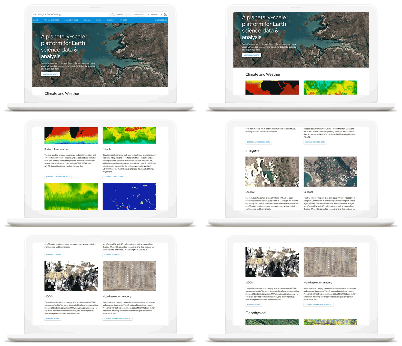
As we work with our customers to accelerate their sustainability initiatives, earth observation data is proving critical to effectively plan for the long-term impacts of climate change. To extend our geospatial and sustainability use cases we’re also expanding our partnerships with CARTO, Climate Engine, Geotab, NGIS, and Planet to bring their data and core applications to Google Cloud.
These partners will each make their existing platforms and datasets available globally on Google Cloud, giving you low-latency and reliable access to critical data and applications that will inform your sustainability initiatives. By integrating water availability, agricultural data, weather risks, and extensive daily satellite imagery into Earth Engine and BigQuery, you can achieve more ambitious goals for the sustainability of your business and our planet.
Committing to help you meet your climate goals
With each of these tools, we’re working to reduce the barriers you face in adopting more sustainable technology practices. We understand that building more sustainable applications and infrastructure is not easy. You face competing priorities, technical challenges, and the perception that climate action is costly.
It doesn’t have to be this way. Today, we are making a sustainability pledge to you: teams across Google Cloud are committing to eliminating the barriers you face in building a more sustainable digital future for your organization, and will help you take action today to realize your climate goals. We’ll do this in a number of ways:
- In digital transformation projects and workshops, sustainability teams will always have a seat at the planning table, so we can work together on using cloud technology to build a more sustainable future.
- We’re putting low-carbon signals natively into our products to help developers choose more sustainable options early in their application development.
- We’ll ensure carbon impact is measured consistently with other key performance indicators. Leveraging the social cost of carbon, the ROI models and value assessments you conduct with Google Cloud will project your emissions impact too.
- We’ll be transparent about our carbon impact, by publishing third-party reviewed reports and methodologies, so you can trust the data for your own reports and disclosures.
- We’ll continue to work with the industry on best practices, including educational resources like Sustainable IT – Decoded, a new masterclass created in partnership with Intel, that shares the expertise of sustainability thought leaders.
For the next decade we need to work together to avert the worst consequences of climate change. We’ve made tremendous progress in building technology that helps everyone do more for the planet, and we’re excited to see what you do with it. Visit this page to learn more about Google Cloud’s sustainability efforts.
New Visual Interface for Google Cloud’s Speech-to-Text API Makes API Easy to Use !

4675
Of your peers have already read this article.
2:00 Minutes
The most insightful time you'll spend today!
At Google Cloud, we’re committed to making artificial intelligence (AI) accessible to everyone and easier to harness for new use cases. That’s why we’re excited to announce the general availability of our intuitive, new visual user interface for Google Cloud’s Speech-to-Text (STT) API, right in Google Cloud Console, which makes the API much simpler and easier for developers to use.
The STT API lets developers convert speech into text by leveraging Google’s years of research in automatic speech recognition and transcription technology. As advancements in AI continue to bring speech to new interfaces and devices, the STT API helps developers add speech functionality to their applications in order to better meet consumer demands.
The STT API covers a wide variety of use cases, from dictation and short commands, to captioning and subtitles. Getting the most of STT, however, can be a complicated process. To achieve the highest accuracy on any AI use case requires careful testing and tuning.
Previously, developers building on the STT API had to do this work manually by carefully experimenting with our API. Just to get started, developers needed familiarity with GCP integration concepts and had to either build their own tools or manage various scripts and API calls to fully understand the API documentation. These actions required cumbersome and time-consuming effort and made measuring, customizing, and improving models even more difficult.
Today’s announcement significantly simplifies the process, facilitating iteration and integration of models into developers’ applications by letting developers perform every API function from within the Google Cloud Console. These tools will make it easier for developers to integrate the STT API with their products or services. This update also gives developers the ability to manage and quickly iterate on their STT model customizations with Model Adaptation.
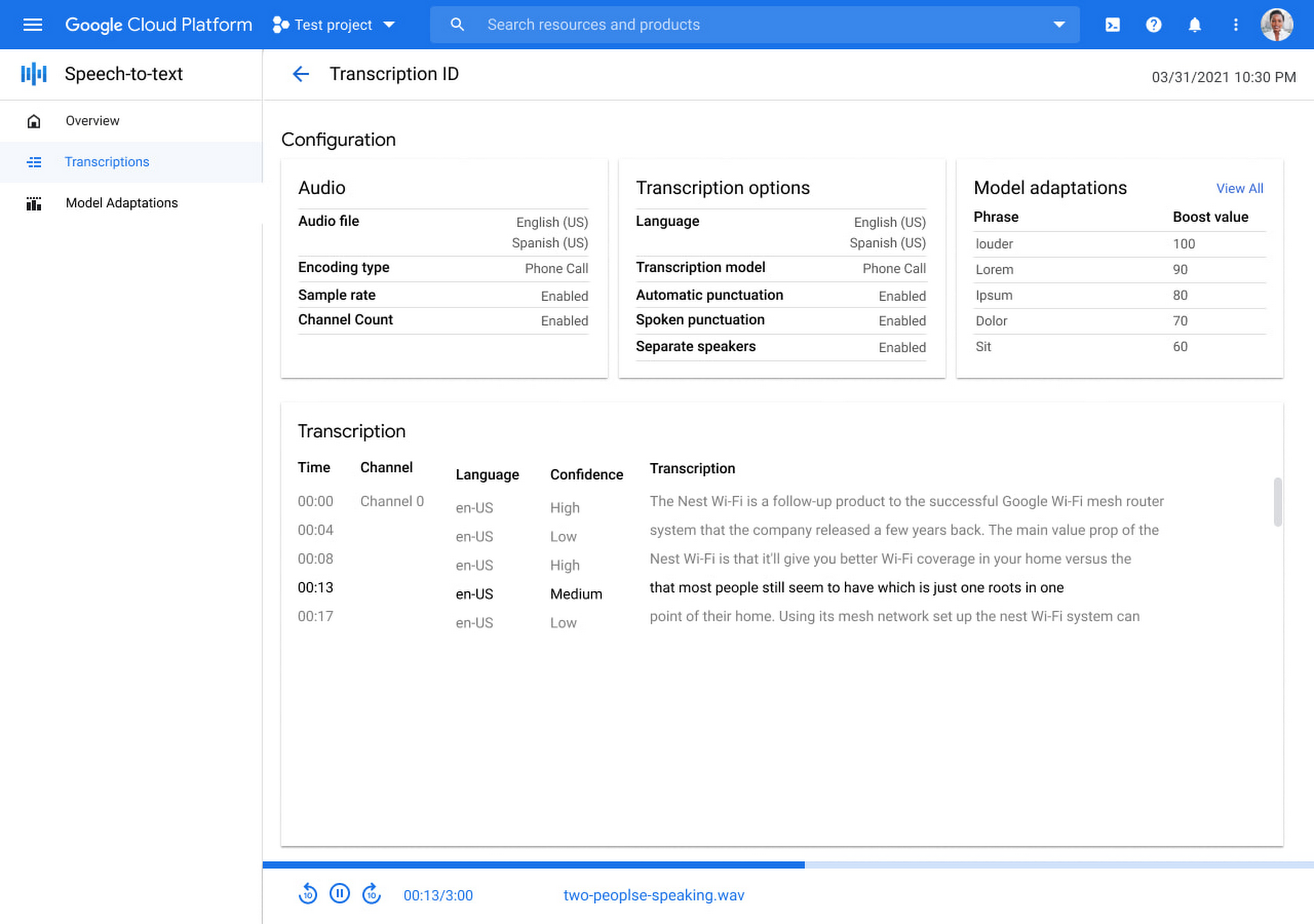
Model Adaptation allows developers to customize STT specifically for their domains or use cases. Developers can maintain lists of words and weights that will be applied to either every request or just single requests, depending on their needs. Model adaptations are reusable and composable, so once developers have seen good results in the STT Cloud Console, they can deploy to their entire solution.
The Speech-to-Text Cloud Console and Model Adaptation API is available now in all Google Cloud regions and languages and is accessible to all GCP users with no additional cost to that of the underlying API usage. The STT API supports over 70 languages in 120 different local variants. If you’re a developer looking for an easy to use, easy to integrate, and high-quality STT experience, sign up for our free trial and try our new interface on your own datasets today!
More Relevant Stories for Your Company

How Kinguin Notched Up Shopping Experience with Google Recommendations AI
Over 2.14 billion people worldwide are expected to buy online this year, according to Statista. Online retail sales will account for 22% of all purchases by 2023. But in a competitive retail landscape, positive interactions can mean the difference between a sale and an abandoned shopping cart. One of the leading global


Supercharge Marketing with Ready-Made, Centralized Smart Analytics
Your company has lots of valuable marketing data, but it’s spread across many systems and teams. That's a problem. In fact, only 13% of organisations feel like they're making the most out of their available customer data today. And the reason is that data--marketing and customer data--is spread across many

Trading and Investment Companies will Increase Consumption of Cloud Services: Study Confirms
While some traditional financial services companies have more slowly transitioned to the cloud, capital markets firms have embraced cloud computing across their entire value chains — front-, middle-, and back-office. We wanted to understand the dynamics behind this rapid adoption, the most common use cases, and the types of technology
Technical deep dive on Looker: The enterprise BI solution for Google Cloud
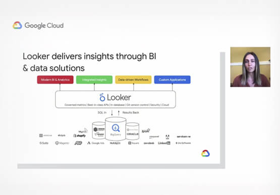
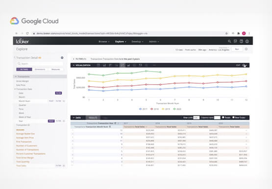
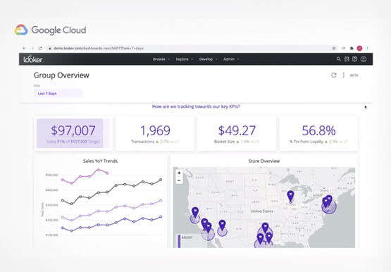
Thousands of users accessing petabytes of data on a daily basis: This is a challenging proposition for enterprises, without a doubt. But Looker makes it possible. Beyond just accessing data though, Looker’s platform transforms your company’s relationship with data. Go under the hood of Looker, with Olivia Morgan, Enterprise CE,
